

NeumannValue
NeumannValue[val,pred]
represents a Neumann boundary value val, specified on the part of the boundary of the region given to NDSolve and related functions where pred is True.
Details
- NeumannValue is used within partial differential equations to specify boundary values in functions such as DSolve and NDSolve.
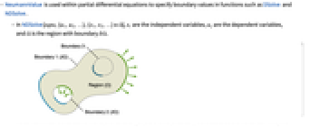
- In NDSolve[eqns,{u1,u2,…},{x1,x2,…}∈Ω], xi are the independent variables, uj are the dependent variables, and Ω is the region with boundary ∂Ω.
- Locations where Neumann values might be specified are shown in green. They appear on the boundary ∂Ω of the region Ω and specify a flux across those edges in the direction of the outward normal.
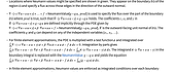
- ∇·(-c ∇u-α u+γ)+…=f+NeumannValue[g-q u,pred] is used to specify the flux over the part of the boundary ∂Ω where pred is true, such that
 ·(c ∇u+α u-γ)=g-q u holds. The coefficients c, α, and γ in
  ·(c ∇u+α u-γ)=g-q u are defined implicitly through the PDE given by ∇·(-c ∇u-α u+γ)+β·∇u+a u=f+NeumannValue[g-q u,pred].
  is the outward-facing unit normal of ∂Ω. The coefficients g and q can depend on any of the independent variables {x1,x2,…}.
 - For finite element approximations, the PDE is multiplied with a test function
 and integrated over
  Integration by parts gives
 . The integrand
  in the boundary integral is replaced with the NeumannValue
  and yields the equation
  . »
. » - In finite element approximations, Neumann values are enforced as integrated conditions over each boundary element in the discretization of ∂Ω where pred is True. Boundary elements are points in 1D, edges in 2D, and faces in 3D.
- When no boundary condition is specified on a part of the boundary ∂Ω, then the flux term ∇·(-c ∇u-α u+γ)+… over that part is taken to be f=f+0=f+NeumannValue[0,…], so not specifying a boundary condition at all is equivalent to specifying a Neumann 0 condition.
- A positive NeumannValue on the right-hand side of an equation models a flux into the domain.
- Any logical combination of equalities and inequalities in the independent variables x1,… may be used for the predicate pred.
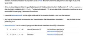
- NeumannValue can be used to specify both Neumann and Robin boundary conditions:
-
 ·(c ∇u+α u-γ)=0
natural (Neumann 0) no conditions specified or NeumannValue[0,pred]  ·(c ∇u+α u-γ)=g
Neumann NeumannValue[g,pred]  ·(c ∇u+α u-γ)=g-q u
Robin (generalized Neumann) NeumannValue[g-q u,pred]  ·(c ∇u+α u-γ)=g-h(u)
generalized nonlinear Neumann NeumannValue[g-h[u],pred] - For systems, ∇·∑j(-cj∇uj-αjuj+γ)+…f+NeumannValue[g-∑jqjuj]+… corresponds to the condition
 being satisfied on the parts of the region boundary where pred is True.
 - For time-dependent equations, both val and pred may depend on time.
- The purpose and meaning of NeumannValue and Derivative in partial differential equations are subtly different. »
- For finite element approximations, NeumannValue operates on nodes in 1D, on edges in 2D and on faces in 3D.
- A DirichletCondition and a NeumannValue should not be specified on the same part of the boundary.
- Several NeumannValue may overlap on the boundary. »
Examples
open all close allBasic Examples (1)
Scope (4)
Solve the nonlinear equation ![]() over a line segment with a generalized Neumann condition
over a line segment with a generalized Neumann condition ![]() for
for ![]() and a Dirichlet condition
and a Dirichlet condition ![]() for
for ![]() :
:
Verify the numeric solution with the analytical solution:
Solve a PDE with a nonlinear generalized Neumann boundary condition on a curved edge.
More than one NeumannValue can be active on the same part of the boundary:
Note the kink at ![]() . In the part below
. In the part below ![]() , both instances of NeumannValue are active, while in the part above
, both instances of NeumannValue are active, while in the part above ![]() , only one NeumannValue is active.
, only one NeumannValue is active.
A NeumannValue can be used to approximate a DirichletCondition.
Solve a PDE with two instances of DirichletCondition and a parameter ![]() for the Dirichlet value:
for the Dirichlet value:
Solve the same PDE with one DirichletCondition replaced by a scaled generalized NeumannValue:
Inspect the difference between the solutions:
This approach to an approximate DirichletCondition with NeumannValue should only be used when there are Dirichlet conditions and Neumann values that need to be accommodated on the same stretch of the boundary.
Applications (12)
1D Problems (2)
Solve ![]() on the unit length with Dirichlet boundary condition
on the unit length with Dirichlet boundary condition ![]() and Robin boundary condition
and Robin boundary condition ![]() :
:
Compare the numerical to the analytical solution:
Solve ![]() on the unit length with Dirichlet boundary condition
on the unit length with Dirichlet boundary condition ![]() and Robin boundary condition
and Robin boundary condition ![]() :
:
Compare the difference of the value of ![]() to the prescribed Dirichlet boundary condition value 1 at
to the prescribed Dirichlet boundary condition value 1 at ![]() :
:
Compare the difference of the value of ![]() to the prescribed Robin boundary condition of
to the prescribed Robin boundary condition of ![]() at
at ![]() :
:
Since this is an integrated condition, how well the condition is satisfied depends on the mesh. Using a finer mesh gives a better result:
2D Problems (2)
Specify a region by boundaries:
Show the region and the boundaries:
Solve a Laplace equation with a temperature set on the red and blue boundaries and a flux over the green boundary:
Neumann boundary conditions can be used to exploit symmetries of a region. Specify a region with a hole:
Set multiple Dirichlet conditions ![]() on the inner and
on the inner and ![]() on the outer boundary:
on the outer boundary:
Solve the equation over a region and visualize the result:
Specify a symmetric subregion:
Zero Neumann conditions are assumed for boundaries with no explicit condition set:
Time-Dependent Problems (4)
Solve a time-dependent problem with initial and boundary conditions:
Solve a wave equation with reflecting boundary conditions:
Solve a wave equation with absorbing boundary conditions:
Solve a wave equation with absorbing boundary conditions. Note that the Neumann value is for the first time derivative of ![]() :
:
Boundary Conditions for Coupled Systems (3)
Specifying a system of coupled equations:
Solve the system of equations with two Dirichlet conditions on the left-hand side and two Neumann conditions on the right-hand side:
Specify a system of coupled differential equations:
Specify Dirichlet and Neumann boundary conditions and solve the system of equations:
Compare the result with an analytical solution:
Plot the error between the numerical and the analytical solutions:
Specify a plane stress operator with Young's modulus and Poisson's ratio over a bar:
The bar is held fixed at the left edge. On the right edge, a boundary load is applied in the negative ![]() direction:
direction:
Contour plot the deformation of the bar in the ![]() direction:
direction:
Properties & Relations (1)
This section explores how setting boundary conditions inside a region affects the solution. The domain is a region from ![]() and has an internal boundary at
and has an internal boundary at ![]() . For this, a finite element boundary mesh is created that has nodes at
. For this, a finite element boundary mesh is created that has nodes at ![]() ,
, ![]() and
and ![]() :
:
To illustrate the behavior of different boundary conditions at an internal boundary, a diffusion type equation has been chosen, where the diffusion coefficient ![]() :
:
As boundary conditions, set specific values at the left and right domain ends:
In the first example, set the PDE equal to 0. That is, there is no other interaction at the internal point at ![]() . This is the default behavior:
. This is the default behavior:
The default behavior is the same as setting a Neumann zero value at ![]() :
:
The difference between the default solution and the Neumann zero solution is zero; they are exactly the same solution:
Next, a specific value of ![]() is set at
is set at ![]() :
:
From the plot, it can be seen that the dependent variable ![]() has a value of
has a value of ![]() at
at ![]() :
:
In the next experiment, a Neumann value of ![]() is set at
is set at ![]() . What this means is not exactly clear, as it is unclear in which direction the normal
. What this means is not exactly clear, as it is unclear in which direction the normal
The plot below compares the various internal boundary conditions:
For further experiments, the diffusion coefficient could be made discontinuous at the internal material boundary by setting ![]() :
:
Alternatively, the values of the boundary conditions can be flipped.
Possible Issues (4)
Exclusively specifying Neumann boundary conditions for stationary PDEs may result in a non-unique solution. In some cases, the system may not be solvable at all:
Specifying a Robin boundary condition is sufficient:
Solve a Laplace equation ![]() with a diffusion coefficient
with a diffusion coefficient ![]() over a rectangle with Dirichlet and Neumann conditions
over a rectangle with Dirichlet and Neumann conditions ![]() for
for ![]() and
and ![]() for
for ![]() :
:
Verify that the solution is consistent with the Neumann value on the right-hand side:
Note that setting a diffusion coefficient ![]() to solve a Laplace equation
to solve a Laplace equation ![]() causes the Neumann value to be
causes the Neumann value to be ![]() :
:
Verify that this solution is also consistent with the Neumann value on the right-hand side:
Not specifying a boundary condition on a part of the boundary implies a natural ![]() boundary condition:
boundary condition:
This is the same boundary condition:
Sometimes, an imported mesh or even a generated mesh may have numerical imprecision. For example, an intended region is a rectangle ![]() , but the discretized version of the region has an imprecision such that one actually has
, but the discretized version of the region has an imprecision such that one actually has ![]() . If in such cases a predicate of the form
. If in such cases a predicate of the form ![]() is specified, an error message will be generated because
is specified, an error message will be generated because ![]() does not exist. Consider this constructed example:
does not exist. Consider this constructed example:
One way to deal with this is to formulate the predicate as a bound ![]() , where
, where ![]() is the thickness of the bound:
is the thickness of the bound:
This technique can also be used for more complicated predicates such as circular parts of a boundary, where the numerical precision issue is more likely to come up.
Text
Wolfram Research (2014), NeumannValue, Wolfram Language function, https://reference.wolfram.com/language/ref/NeumannValue.html (updated 2023).
CMS
Wolfram Language. 2014. "NeumannValue." Wolfram Language & System Documentation Center. Wolfram Research. Last Modified 2023. https://reference.wolfram.com/language/ref/NeumannValue.html.
APA
Wolfram Language. (2014). NeumannValue. Wolfram Language & System Documentation Center. Retrieved from https://reference.wolfram.com/language/ref/NeumannValue.html