

NDEigenvalues
NDEigenvalues[ℒ[u[x,y,…]],u,{x,y,…}∈Ω,n]
gives the n smallest magnitude eigenvalues for the linear differential operator ℒ over the region Ω.
NDEigenvalues[{ℒ1[u[x,y,…],v[x,y,…],…],ℒ2[u[x,y,…],v[x,y,…],…],…},{u,v,…},{x,y,…}∈Ω,n]
gives eigenvalues for the coupled differential operators {op1,op2,…} over the region Ω.
NDEigenvalues[eqns,{u,…},t,{x,y,…}∈Ω,n]
gives the eigenvalues in the spatial variables {x,y,…} for solutions u,… of the coupled time-dependent differential equations eqns.
Details and Options
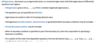
- NDEigenvalues, also known as an eigenmode solver, is a numerical eigen solver that finds eigenvalues of differential equations over regions.
- NDEigenvalues gives a list {λ1,…,λn} of the n smallest magnitude eigenvalues λi.
- The equations eqns are specified as in NDSolve.
- Eigenvalues are sorted in order of increasing absolute value.
- Homogeneous DirichletCondition, NeumannValue or generalized Robin boundary conditions may be included. »
- PeriodicBoundaryCondition may be included.
- When no boundary condition is specified on part of the boundary ∂Ω, then this is equivalent to specifying a Neumann 0 condition.
- For a system of first-order time-dependent equations, the time derivatives D[u[t,x,y,…],t],D[v[t,x,y,…],t],… are effectively replaced with λ u[x,y,…],λ v[x,y,…],….
- Systems of time-dependent equations that are higher than first order are reduced to a coupled first-order system with intermediate variables ut=u*,
 =…, vt=v*,
 =…, …. Only the functions u, v, … are returned. »
 - NDEigenvalues accepts a Method option that may be used to control different stages of the solution. With Method->{s1->m1,s2->m2,…}, stage si is handled by method mi. When stages are not given explicitly, NDEigenvalues tries to automatically determine what stage to apply a given method to.
- Possible solution stages are:
-
"PDEDiscretization" discretization of spatial operators. "Eigensystem" computation of the eigensystem from the discretized system. "VectorNormalization" normalization of the eigenvectors that are used to construct the eigenfunctions.
Examples
open all close allBasic Examples (3)
Scope (12)
1D (7)
Specify homogeneous Dirichlet boundary conditions:
Find the 4 smallest eigenvalues:
Specify homogeneous Neumann boundary conditions:
Find the four smallest eigenvalues:
Specify a transient equation with homogeneous Dirichlet boundary conditions:
Find the 4 smallest eigenvalues:
Specify a wave equation with homogeneous Dirichlet boundary conditions:
Find the 4 smallest eigenvalues:
Compute the eigenvalues of a generalized wave equation ![]() :
:
Compare to the exact solution of an equivalent first-order system of ordinary differential equations:
Compute the 4 smallest eigenvalues:
Compare the eigenvalues with the analytical eigenvalues:
Write a function to compute parametric, complex-valued periodic eigenvalues of the Laplace operator:
2D (5)
Find the 4 smallest eigenvalues:
Find the 4 smallest eigenvalues of the operator in a unit disk:
Specify a Laplacian operator with homogeneous Dirichlet boundary conditions:
Find the 9 smallest eigenvalues in a rectangle:
Specify a wave equation with homogeneous Dirichlet boundary conditions:
Options (6)
Method (6)
"Eigensystem" (4)
Specify a method to use for finding the eigenvalues:
In this case, the default method is faster:
Arnoldi is used as the default method:
Specify a maximum number of iterations for the Arnoldi method:
Find two eigenvalues of a Sturm–Liouville operator within the band of ![]() with the FEAST method for Eigenvalues:
with the FEAST method for Eigenvalues:
According to the Sturm–Liouville theory, the eigenvalues must be distinct, but for this example they are close to degenerate:
The interval end points ![]() are not included in the interval FEAST finds eigenvalues in; for more information, please refer to the Eigenvalues reference page.
are not included in the interval FEAST finds eigenvalues in; for more information, please refer to the Eigenvalues reference page.
The usage of the "Shift" option is explained in an example below.
"PDEDiscretization" (1)
Change the MaxCellMeasure for the underlying computation:
The exact eigenvalues are 0,1,4,9,…, so the eigenvalue error is:
Applications (4)
Acoustics (1)
Compute the acoustic eigenvalues and eigenfunctions for an approximation of a cross section through a Mini. Import an image of the cross section:
Properties & Relations (3)
Specify a transient equation with homogeneous Dirichlet boundary conditions:
Find the 4 smallest eigenvalues:
Compare an analytical solution to a higher-order time-dependent PDE.
Find the six smallest eigenvalues of a wave equation ![]() for
for ![]() between 0 and
between 0 and ![]() :
:
Compare the eigenvalues with the exact solution of ![]() transformed into a system of two first-order equations:
transformed into a system of two first-order equations:
Show the relation between higher-order time-dependent PDEs and systems of first-order PDEs.
Find the six smallest eigenvalues of a wave equation ![]() within 0 and
within 0 and ![]() :
:
Find the six smallest eigenvalues of a wave equation given as a system of first-order PDEs ![]() :
:
The eigenvalues for the second-order system and the system of first-order equations are the same:
Possible Issues (10)
The computed eigenvalues depend on the granularity of the discretization:
The exact eigenvalues are 0,1,4,9,…, so the eigenvalue error is:
A finer mesh results in a decreased discretization error:
The eigenvalues of the wave equation will be the square root of the angular frequencies:
Compare to the exact solution of an equivalent first-order system of ordinary differential equations:
Eigenvalues with inhomogeneous Dirichlet conditions cannot be solved for:
Eigenvalues with homogeneous Dirichlet conditions can be solved for:
Eigenvalues with inhomogeneous Neumann values cannot be solved for:
Eigenvalues with homogeneous Neumann values can be solved for:
Eigenvalues with inhomogeneous generalized Neumann values cannot be solved for:
The operator and possible boundary conditions need to be stationary and linear:
Initial conditions will be set to zero and ignored:
NDEigenvalue converts PDEs to time-dependent PDEs. This transformation is not unique and may lead to what seem to be unexpected results for coupled PDEs:
Internally, the given equations are rewritten as a system of time-dependent PDEs. In the previous case from the given dependent variables {v[x],u[x]}, the following temporal system is generated: {D[v[t, x], t] == - u[t, x] - Laplacian[u[t, x], {x}],D[u[t, x], t] == -v[t, x] - Laplacian[v[t, x], {x}]}
To uniquely specify the system of equations, it is best to use the temporal description:
More information on this topic can be found in Finite Element Method Usage Tips.
In some cases, NDEigenvalues may return what seem to be unexpected results for coupled PDEs:
One way to avoid this issue is to specify an ordering of the dependent variables via the "InterpolationOrder" option:
Alternatively, the "Direct" method can be used:
More information on this topic can be found in Finite Element Method Usage Tips.
NDEigenvalues finds the ![]() smallest magnitude eigenvalues for a given linear differential operator. Particularly in cases where one is interested in finding the most negative eigenvalues, e.g. many quantum mechanical problems, the
smallest magnitude eigenvalues for a given linear differential operator. Particularly in cases where one is interested in finding the most negative eigenvalues, e.g. many quantum mechanical problems, the ![]() most negative eigenvalues might not correspond with the
most negative eigenvalues might not correspond with the ![]() eigenvalues NDEigenvalues returns by default. To see this, consider the following example.
eigenvalues NDEigenvalues returns by default. To see this, consider the following example.
Take, for instance, the dimensionless radial Schrödinger equation for the hydrogen atom, where the energy units are Rydbergs and length is measured in Bohr radii.
Define the radial Schrödinger equation:
Solve the eigenvalue problem for ![]() . A refined mesh is used for a good approximation quality:
. A refined mesh is used for a good approximation quality:
Look at the eigenvalues obtained in electronvolts:
These correspond to the eigenvalues closest to ![]() . But they are not in the desired order. For instance, take a look at the analytical eigenvalues for this problem.
. But they are not in the desired order. For instance, take a look at the analytical eigenvalues for this problem.
The analytical energies for this equation follow the following relation:
If you know in advance a lower bound for the eigenvalues, say ![]() , you can redefine the eigenvalue problem
, you can redefine the eigenvalue problem ![]() as
as ![]() . In other words, a new eigenvalue problem:
. In other words, a new eigenvalue problem: ![]() , where
, where ![]() and
and ![]() . Given that
. Given that ![]() is a negative lower bound for
is a negative lower bound for ![]() , the shift ensures that
, the shift ensures that ![]() will only assume positive values. Therefore, the
will only assume positive values. Therefore, the ![]() smallest magnitude values of
smallest magnitude values of ![]() will correspond to the
will correspond to the ![]() most negative values of
most negative values of ![]() . That way, one can calculate for
. That way, one can calculate for ![]() and then get
and then get ![]() . The easiest way to do this is to use the "Shift" option.
. The easiest way to do this is to use the "Shift" option.
Define a shift and solve the eigenvalue problem:
Look at the eigenvalues obtained in electronvolts:
These correspond to the most negative eigenvalues, but in reverse order, and then it is necessary to sort the eigenstates.
Sort the eigenstates with Sort:
Take a look at the difference between the analytical eigenvalues and the obtained results:
Text
Wolfram Research (2015), NDEigenvalues, Wolfram Language function, https://reference.wolfram.com/language/ref/NDEigenvalues.html.
CMS
Wolfram Language. 2015. "NDEigenvalues." Wolfram Language & System Documentation Center. Wolfram Research. https://reference.wolfram.com/language/ref/NDEigenvalues.html.
APA
Wolfram Language. (2015). NDEigenvalues. Wolfram Language & System Documentation Center. Retrieved from https://reference.wolfram.com/language/ref/NDEigenvalues.html