D 
D[f,x]
gives the partial derivative ![]() .
.
D[f,{x,n}]
gives the multiple derivative ![]() .
.
D[f,x,y,…]
gives the partial derivative ![]() .
.
D[f,{x,n},{y,m},…]
gives the multiple partial derivative ![]() .
.
D[f,{{x1,x2,…}}]
for a scalar f gives the vector derivative ![]() .
.
D[f,{array}]
gives an array derivative.
Details and Options
- D is also known as derivative for univariate functions.
- By using the character ∂, entered as
 pd
pd or \[PartialD], with subscripts, derivatives can be entered as follows:
 -
D[f,x] ∂xf D[f,{x,n}] ∂{x,n}f D[f,x,y] ∂x,yf D[f,{{x,y}}] ∂{{x,y}}f - The comma can be made invisible by using the character \[InvisibleComma] or
 ,
, .
. - The partial derivative D[f[x],x] is defined as
 , and higher derivatives D[f[x,y],x,y] are defined recursively as
  etc.
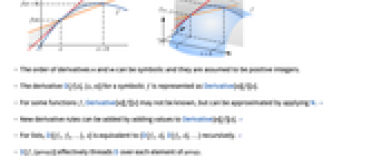
etc. - The order of derivatives n and m can be symbolic and they are assumed to be positive integers.
- The derivative D[f[x],{x,n}] for a symbolic f is represented as Derivative[n][f][x].
- For some functions f, Derivative[n][f][x] may not be known, but can be approximated by applying N. »
- New derivative rules can be added by adding values to Derivative[n][f][x]. »
- For lists, D[{f1,f2,…},x] is equivalent to {D[f1,x],D[f2,x],…} recursively. »
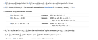
- D[f,{array}] effectively threads D over each element of array.
- D[f,{array,n}] is equivalent to D[f,{array},{array},…], where {array} is repeated n times.
- D[f,{array1},{array2},…] is normally equivalent to First[Outer[D,{f},array1,array2,…]]. »
- Common array derivatives include:
-
D[f,{{x1,x2,…}}] gradient {D[f,x1],D[f,x2],…} D[f,{{x1,x2,…},2}] Hessian {{D[f,x1,x1],D[f,x1,x2],…},{D[f,x2,x1],D[f,x2,x2],…},…} D[{f1,f2,…},{{x1,x2,…}}] Jacobian {{D[f1,x1],D[f1,x2],…},
{D[f2,x1],D[f2,x2],…},…} - If f is a scalar and x={x1,…}, then the multivariate Taylor series at x0={x01,…} is given by:
 ,
,- where fi=D[f,{x,i}]/.{x1x01,…} is an array with tensor rank
 . »
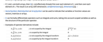
. » - If f and x are both arrays, then D[f,{x}] effectively threads first over each element of f, and then over each element of x. The result is an array with dimensions Join[Dimensions[f],Dimensions[x]]. »
- VectorSymbol, MatrixSymbol or ArraySymbol can be used to indicate that variables or function values are vectors, matrices or arrays.
- D can formally differentiate operators such as integrals and sums, taking into account scoped variables as well as the structure of the particular operator.
- Examples of operator derivatives include:
-

 is not scoped by the integral

 is scoped by the integral

 is not scoped by the integral transform

 is scoped by by the integral transform
- All expressions that do not explicitly depend on the variables given are taken to have zero partial derivative.
- The setting NonConstants{u1,…} specifies that ui depends on all variables x, y, etc. and does not have zero partial derivative. »
Examples
open allclose allBasic Examples (7)
Scope (89)
Basic Uses (12)
Derivative of an expression with respect to x:
Derivative of an expression at a point:
Derivative of a function at a general point x:
This can also be achieved using fluxion notation:
This can be found more easily using fluxion notation:
The third derivative at the point x==-1:
Derivative involving symbolic functions:
Partial derivatives of an expression with respect to x and y:
The mixed partial derivative ![]() :
:
The mixed partial derivative ![]() :
:
Differentiate with respect to a compound expression:
Differentiate with respect to different compound expressions:
Derivative of a vector expression:
Vector derivative of an expression, also known as the gradient:
Symbolic Functions (9)
Derivative of a symbolic function:
Substitute in a pure function for f to get a particular result:
The chain rule for composite functions:
Product rule for three functions:
State the rule using an Inactive derivative:
Partial derivative of a symbolic function:
Substitute in for f a pure function in two variables:
Derivative of a pure function with respect to non-argument parameters:
The result is the function that at point x gives the derivative of ![]() with respect to a:
with respect to a:
Local variables are independent from the differentiation variable:
Derivative of a symbolic function at a point:
The same, using prime notation:
Derivative of an inverse function:
Elementary Functions (6)
Special Functions (8)
The logarithmic derivative of Gamma is the PolyGamma function:
Derivatives of Airy functions are given in terms of AiryAiPrime and AiryBiPrime:
The derivative of Zeta has a closed-form expression at the origin:
Special functions with elementary derivatives:
Special functions with derivatives expressed in terms of the same functions:
Derivative of JacobiSN:
Derivative of JacobiCD:
Derivative of LogIntegral:
Derivative of ExpIntegralEi:
Derivative of order n for SinIntegral:
Piecewise and Generalized Functions (8)
Derivative of a piecewise function:
Derivative of a ConditionalExpression:
Convert a symbolic function into a piecewise function over the reals to differentiate it:
Compute the piecewise derivative over a finite range:
Classical derivatives of pointwise-defined engineering functions:
Distributional derivatives of generalized functions:
Derivative of RealAbs:
Their counterparts on the complex plane are nowhere differentiable:
Derivative of Floor:
Implicitly Defined Functions (3)
Vector-Valued Functions (5)
The first derivative to a vector-valued function at a general value t:
Computing the same using prime notation:
Computing the same using prime notation:
The derivative of a vector-valued function stored as a SparseArray:
Convert the result to a normal array:
The derivative of matrix represented as a SymmetrizedArray object:
Vector Argument Functions (6)
Gradient of a scalar function:
Jacobian of a vector-valued function:
Second-order derivative tensor:
Compute the derivative of the determinant with respect to the original matrix:
The gradient of a vector-valued function stored as a SparseArray:
The result is another SparseArray, containing only the nonzero entries:
Convert the result to a normal matrix:
Hessian computed as a SparseArray:
The gradient can also be computed as a SparseArray, but in this case it is effectively dense:
Jacobian computed as a SparseArray:
Symbolic Array Arguments and Functions (8)
Derivative of a symbolic vector-valued function with respect to a scalar argument:
Derivative of a symbolic matrix–valued function with respect to a scalar argument:
Derivative of a symbolic array–valued function with respect to a scalar argument:
Derivatives of scalar-valued functions with respect to symbolic vector arguments:
Real symbolic vector argument:
Derivatives of scalar-valued functions with respect to symbolic matrix arguments:
Real symbolic matrix argument:
Derivative of a scalar-valued function with respect to a symbolic array argument:
Derivatives of symbolic array–valued functions with respect to symbolic array arguments:
Integrals and Integral Transforms (6)
Differentiate unevaluated integrals:
Differentiate the Inactive form of an integral to get the fundamental theorem of calculus:
A more general form of the fundamental theorem:
Differentiate an inactive FourierTransform:
Sums and Summation Transforms (4)
Differentiate an unevaluated sum:
Differentiation with respect to the dummy variable gives zero:
Differentiate the Inactive form of a sum:
Differentiate an inactive GeneratingFunction:
Indexed Differentiation (9)
Differentiate with respect to an indexed variable, introducing KroneckerDelta factors:
Use Inactive to prevent expansion of the sum:
Summation indices will be renamed if needed, to avoid name ambiguities:
Differentiate an inactive table with respect to an indexed variable:
Activate the result to get the explicit vector result:
Differentiate an inactive table twice with respect to an indexed variable:
In this case only the j![]() entry is nonzero:
entry is nonzero:
Use any notation for indexed variables in sums and tables:
Differentiate with respect to a symbolic table of indexed variables:
Activating the result gives the explicit gradient:
Differentiate twice with respect to a symbolic table of indexed variables, introducing a dummy index:
Replace symbolic variables with explicit values:
Use symbolic vector differentiation of another symbolic vector:
Vector differentiation of a vector with respect to itself gives the identity matrix:
Functions Defined by Derivatives (5)
Define the derivative with prime notation:
This rule is used to evaluate the derivative:
Define the derivative at a point:
Prescribe values and derivatives of f and g:
Find the derivative of the composition at x=3:
Define a partial derivative with Derivative:
Options (1)
Applications (47)
Geometry of the Derivative (5)
The derivative gives the slope of the tangent line at a point:
For small displacements h from the base point π, the tangent line gives an excellent approximate of f:
The tangent and f are visually indistinguishable from each other over a small, and only a small, plot range:
The derivative gives the limit of the slope of the secant line connecting {x,f[x]} to {x+h,f[x+h]}:
Visualize the process for the point {1,f[1]}:
Find an equation for the tangent line to a function:
General equation for the tangent line at x=a:
Find an equation for the normal line to a function:
General equation for the normal line at x=a:
Find equations for the tangent lines to a function that pass through a point:
Characterization of Functions (5)
Find the turning points on a plane curve:
Find the critical points of a function:
By the second derivative test, these are all maxima or minima:
Visualize the critical points:
Find all values of c that satisfy the Mean Value theorem on an interval:
Define the secant line from a to b:
Define the tangent lines associated with the two values of c:
Visualize the two tangent lines parallel to the secant line along with the original function:
Use the first derivative to characterize a function:
Find the critical points of a function:
Find where the function is increasing:
Find where the function is decreasing:
Use the second derivative to characterize a function:
Find the inflection points of a function:
Find where the function has positive concavity:
Relation to Integration (2)
Multivariate and Vector Calculus (6)
Find the critical points of a function of two variables:
Compute the signs of ![]() and the determinant of the second partial derivatives:
and the determinant of the second partial derivatives:
By the second derivative test, the first two points—red and blue in the plot—are minima and the third—green in the plot—is a saddle point:
Find the curvature of a circular helix with radius r and pitch c:
Obtain the same result using ArcCurvature:
Compute a univariate Taylor series by hand:
Compute a multivariate Taylor series by hand:
Write a function to automate the process:
Recompute the above using the new function:
The gradient vector can be computed by finding the partial derivatives of a function:
Find the gradient vector of the function ![]() :
:
Visualize the direction of the gradient vector using a unit vector representation:
The curl of a vector field on the plane can be computed by subtracting the derivatives of its components:
Find the curl of the vector field ![]() :
:
Visualize the 2D curl as the net "rotation" of the vector field at a point, with red and green representing clockwise and counterclockwise curl, respectively, and radius proportional to the magnitude of rotation:
The divergence of a vector field can be computed by summing the derivatives of its components:
Find the divergence of a 2D vector field:
Visualize 2D divergence as the net "flow" of the vector field at a point, with red and green representing outflow and inflow, respectively, and radius proportional to the magnitude of the flow:
Differential Equations (6)
Construct the differential equation satisfied by an implicit function y[x]:
Use D to specify ordinary and partial differential equations:
These can be solved using DSolve:
Define a wave equation in two spatial variables:
Define initial values for the function and its first time derivative:
Solve the system using DSolve:
Extract a few terms from the Inactive sum:
The two-dimensional wave executes periodic motion in the vertical direction:
Specify a Laplacian operator using D:
Specify homogeneous Dirichlet boundary conditions:
Find the 4 smallest eigenvalues and eigenfunctions of the operator in a unit disk:
Specify an integro-differential equation using D:
Specify an initial condition to obtain a particular solution:
Plot the solutions for different values of a:
Find a second-degree polynomial solution to the differential equation:
Rates of Change (5)
The height of a projectile at time t is given by:
Compute the acceleration at t:
Find when the projectile reaches its maximum height:
Find the maximum height of the projectile:
The area of a circle as a function of time is given by:
Compute the rate of change of area:
Find the rate of change of area at a radius of 10 m if the radius increases at a rate of 5m/s:
The position of a particle is given by:
Compute the velocity, acceleration, jerk, snap (jounce), crackle and pop of the particle:
The total resistance in a circuit of two resistors connected in parallel is given by:
Calculate RT for the given values of R1 and R2:
Find the rate of change of the total resistance:
Calculate the rate of change of the total resistance with the given values:
Volume of a cube in terms of side length l is given by:
Surface area of a cube is given by:
Compute the rate of change of the volume of a cube with respect to surface area using the chain rule:
Solve for l in terms of surface area and substitute that into the result:
Implicit Functions (3)
Optimization (3)
Find the maximum area of a rectangular fence of 2000 ft., bordered on one side by a barn:
Compute the area in terms of width:
By the second derivative test, this value is a true maximum:
Alternately, compute the area in terms of length:
Visualize how the area changes as the length changes:
Find the shortest distance from a curve to the point (1,5):
Compute the distance in terms of y:
By the second derivative test, this is a minimum:
Visualize how the distance changes with position:
Find the dimensions of a lidless, cylindrical can with the least material that can hold up to 2 L of water:
Compute the height in terms of the radius, using the volume constraint:
Compute the surface area in terms of the radius:
The radius corresponding to the minimum surface area:
By the second derivative test, this is a minimum:
Compute the radius, height and surface area of the minimum configuration:
L'Hôpital's Rule (3)
Find the limit of the ratio of two functions as x0:
Directly solving the limit leads to an indeterminate form of type ![]() :
:
L'Hôpital's rule can be used because in an interval around ![]() , both
, both ![]() and
and ![]() are defined, and
are defined, and ![]() :
:
Indeed, ![]() and
and ![]() are continuous, and
are continuous, and ![]() , so
, so ![]() can be computed trivially:
can be computed trivially:
Verify the result using Limit:
Visualize the two functions and their ratio:
Find the limit of the ratio of two functions as x∞:
Directly solving the limit leads to an indeterminate form of type ![]() :
:
L'Hôpital's rule can be used because for all ![]() , both
, both ![]() and
and ![]() are defined, and
are defined, and ![]() :
:
However, using the first derivatives also leads to an indeterminate form:
The second derivatives are constant and obviously satisfy the conditions of L'Hôpital's rule:
Hence ![]() can be computed trivially:
can be computed trivially:
Verify the result using Limit:
Find the limit of the product of two functions as x0:
Directly solving the limit leads to an indeterminate form of type 0×∞:
However, ![]() exists and is positive for all
exists and is positive for all ![]() , and it also exists and is negative for all
, and it also exists and is negative for all ![]() :
:
As ![]() is clearly defined for all real
is clearly defined for all real ![]() , L'Hôpital's rule can be applied in the form:
, L'Hôpital's rule can be applied in the form:
The quotient in the right-hand limit gives a continuous expression whose limit is simple to compute:
Symbolic Array Calculus (6)
Approximate the variance for a perturbed vector:
Since the second derivative does not depend on ![]() , the order two approximation equals the exact value:
, the order two approximation equals the exact value:
Approximate the determinant of a perturbed matrix:
Derive a least-squares solution for data ![]() given as a list of pairs
given as a list of pairs ![]() :
:
Find the vector of vertical deviations ![]() for the data:
for the data:
Define the sum of squares of the vertical deviations for the data:
Set up the least-squares equations:
Solve the least-squares problem for this data:
Find GammaDistribution parameters that best fit the given data using the maximum likelihood method:
Maximize the log-likelihood function ![]() :
:
Find a zero of the gradient, with ![]() replaced by
replaced by ![]() :
:
Compare with the result computed using EstimatedDistribution:
Find an optimality condition for a portfolio optimization problem with the expected return ![]() and standard deviation
and standard deviation ![]() :
:
The goal is to maximize ![]() when the vector
when the vector ![]() of asset weights satisfies Total[x]=1. The constraint can be used to represent
of asset weights satisfies Total[x]=1. The constraint can be used to represent ![]() where the unconstrained vector variable
where the unconstrained vector variable ![]() consists of the first
consists of the first ![]() coordinates of
coordinates of ![]() :
:
The maximum occurs at a critical point of ![]() :
:
Express the condition in terms of ![]() :
:
Compute the gradient of the log-likelihood function of the linear regression model represented by the equation ![]() , where
, where ![]() are normally distributed random variables with mean zero and variance
are normally distributed random variables with mean zero and variance ![]() :
:
The log-likelihood function ![]() is given by:
is given by:
Properties & Relations (23)
The derivative of a function is defined as a limit:
The Limit of DifferenceQuotient is the derivative D:
D is the inverse of Integrate:
The fundamental theorem of calculus:
Differentiation inside of Integrate:
D returns formal results in terms of Derivative:
D differentiates expressions with respect to a given variable:
Derivative is an operator and returns pure-function results:
The derivative of a function at a point may not be available in closed form:
An approximation to the derivative can be obtained using N:
D[f,{array1},…] is essentially equivalent to First[Outer[D,{f},array1,…]]:
If f and a are arrays, Dimensions[D[f,{a}]==Join[Dimensions[f],Dimensions[a]]:
D[f,{{x1,x2,…,xn}}] is effectively equivalent to Grad[f,{x1,x2,…,xn}]:
Div[{f1,f2,…,fn},{x1,x2,…,xn}] is the trace of the vector derivative of f:
More generally, Div[f,x] is the contraction of the last two dimensions of the vector derivative of f:
Curl[f,x] is ![]() times the HodgeDual of the vector derivative of f, where r is the rank of f:
times the HodgeDual of the vector derivative of f, where r is the rank of f:
For scalar f, Laplacian[f,{x1,x2,…,xn}] is the trace of the second vector derivative of f:
More generally, Laplacian[f,x] is the contraction of the last two dimensions of the second vector derivative of f:
Compute the derivative of Total[a] with respect to a using symbolic arrays:
Compare with the results obtained using indexed differentiation:
ArcCurvature can be defined in terms of D:
Systems of differential equations involving D can be solved with DSolve:
Use D to specify a heat equation with homogeneous Dirichlet boundary conditions:
The eigensystem for this differential system can be found with DEigensystem:
D can be defined using DifferenceDelta:
D can be defined using DiscreteShift:
The right one-sided derivative is computed with a right-hand limit:
The left one-sided derivative is computed with a left-hand limit:
Note that this function is not differentiable at x==0:
D assumes that other variables are independent of the differentiation variable:
Dt assumes that other variables may depend on the differentiation variable:
By manually specifying all other variables as constant, Dt can yield the same result as D:
Compute the derivative of an implicit function using D and Solve:
Use ImplicitD to compute the derivative of an implicit function:
Possible Issues (5)
Results may not immediately be given in the simplest possible form:
Functions given in different forms can yield the same derivatives:
D returns generic results that may not account for discontinuities, cusps or other special points:
Neither f nor g is differentiable at 0:
f is discontinuous, and g has a cusp:
If a function can be expanded into a Piecewise expression, D will provide more accurate results:
Cached values for D may miss changes in underlying definitions:
The issue can be resolved by clearing the system cache:
The variable of differentiation is treated literally:
The following mathematically equivalent input gives 0 because there is no Sin[x] in the first argument:
Interactive Examples (2)
Text
Wolfram Research (1988), D, Wolfram Language function, https://reference.wolfram.com/language/ref/D.html (updated 2024).
CMS
Wolfram Language. 1988. "D." Wolfram Language & System Documentation Center. Wolfram Research. Last Modified 2024. https://reference.wolfram.com/language/ref/D.html.
APA
Wolfram Language. (1988). D. Wolfram Language & System Documentation Center. Retrieved from https://reference.wolfram.com/language/ref/D.html