

DiscreteLQRegulatorGains
DiscreteLQRegulatorGains[sspec,wts,τ]
gives the discrete-time state feedback gains with sampling period τ for the continuous-time system specification sspec that minimizes a cost function with weights wts.
DiscreteLQRegulatorGains[…,"prop"]
gives the value of the property "prop".
Details and Options
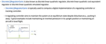


- DiscreteLQRegulatorGains is also known as discrete linear quadratic regulator, discrete linear quadratic cost equivalent regulator or discrete linear quadratic emulated regulator.
- DiscreteLQRegulatorGains is typically used to compute a digital implementation of a regulating controller or tracking controller.
- A regulating controller aims to maintain the system at an equilibrium state despite disturbances
 pushing it away. Typical examples include maintaining an inverted pendulum in its upright position or maintaining an aircraft in level flight.
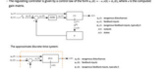
 - The regulating controller is given by a control law of the form
 , where
  is the computed gain matrix.
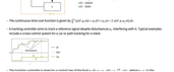
 - The continuous-time cost function is given by
 .
. - A tracking controller aims to track a reference signal despite disturbances
 interfering with it. Typical examples include a cruise control system for a car or path tracking for a robot.
 - The tracking controller is given by a control law of the form
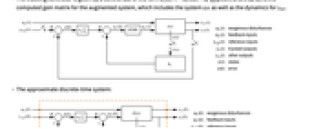
 , where
  is the computed gain matrix for the augmented system, which includes the system sys as well as the dynamics for
  .
. - The approximate discrete-time system:
- The continuous-time cost function is given by
 , where
  are the augmented states.
 - The number of augmented states is given by
 , where
  is given by SystemsModelOrder of sys,
  the order of yref and
  the number of signals yref.
 - The choice of weighting matrices results in a tradeoff between performance and control effort, and a good design is arrived at iteratively. Their starting values can be diagonal matrices with entries
![TemplateBox[{{1, /, z}, i, 2}, Subsuperscript]](Files/DiscreteLQRegulatorGains.en/21.png "TemplateBox[{{1, /, z}, i, 2}, Subsuperscript]") , where zi is the maximum admissible absolute value of the corresponding xi or ui.
, where zi is the maximum admissible absolute value of the corresponding xi or ui. - DiscreteLQRegulatorGains computes the discrete-time controller using an approximated discrete-time equivalent of a continuous-time cost function.
- The discrete-time approximated cost function is
![sum_(k=0)^infty(x^^(k).phi.x^^(k)+TemplateBox[{{{u, _, f}, (, k, )}}, ConjugateTranspose].rho.u_f(k)+2 TemplateBox[{{{x, ^, ^}, (, k, )}}, ConjugateTranspose].psi.u_f(k))](Files/DiscreteLQRegulatorGains.en/22.png "sum_(k=0)^infty(x^^(k).phi.x^^(k)+TemplateBox[{{{u, _, f}, (, k, )}}, ConjugateTranspose].rho.u_f(k)+2 TemplateBox[{{{x, ^, ^}, (, k, )}}, ConjugateTranspose].psi.u_f(k))") , with the following terms:
, with the following terms: -
state weight matrix 
input weight matrix 
cross-coupling weight matrix 
state vector  for regulation and
  for tracking
 - The weights wts can have the following forms:
-
{q,r} cost function with no cross-coupling {q,r,p} cost function with cross-coupling matrix p - The system specification sspec is the system sys together with the uf, yt and yref specifications.
- The system sys can be given as StateSpaceModel[{a,b,c,d}], where a, b, c and d represent the state, input, output and feed-through matrices in the continuous-time system
 .
. - The discrete-time design model dsys is a zero-order hold approximation
 with the following terms:
 -
state matrix 
input matrix 
- The system specification sspec can have the following forms:
-
StateSpaceModel[…] linear control input and linear state AffineStateSpaceModel[…] linear control input and nonlinear state NonlinearStateSpaceModel[…] nonlinear control input and nonlinear state SystemModel[…] general system model <…> detailed system specification given as an Association - The detailed system specification can have the following keys:
-
"InputModel" sys any one of the models "FeedbackInputs" All the feedback inputs uf "TrackedOutputs" None the tracked outpus yt "TrackedSignal" Automatic the dynamics of yref - The feedback inputs can have the following forms:
-
{num1,…,numn} numbered inputs numi used by StateSpaceModel, AffineStateSpaceModel and NonlinearStateSpaceModel {name1,…,namen} named inputs namei used by SystemModel All uses all inputs - For nonlinear systems such as AffineStateSpaceModel, NonlinearStateSpaceModel and SystemModel, the system will be linearized around its stored operating point.
- DiscreteLQRegulatorGains[…,"Data"] returns a SystemsModelControllerData object cd that can be used to extract additional properties using the form cd["prop"].
- DiscreteLQRegulatorGains[…,"prop"] can be used to directly give the value of cd["prop"].
- Possible values for properties "prop" include:
-
"BlockDiagram" sampled-data block diagram of csys "ClosedLoopSystem" sampled-data closed-loop system csys {"ClosedLoopSystem",cspec} detailed control over the form of csys "Design" type of controller design "DesignModel" model used for the design "DiscreteTimeBlockDiagram" block diagram of dcsys "DiscreteTimeClosedLoopPoles" poles of "DiscreteTimeClosedLoopSystem" "DiscreteTimeClosedLoopSystem" dcsys {"DiscreteTimeClosedLoopSystem",cspec} detailed control over the form of dsys "DiscreteTimeControllerModel" dcm "DiscreteTimeDesignModel" approximated discrete-time model dsys "DiscreteTimeFeedbackGainsModel" dgm or {dgm1,dgm2} "DiscreteTimeOpenLoopPoles" poles of dsys "DiscreteTimeWeights" weights ϕ, ρ, π of the approximated cost "FeedbackGains" gain matrix κ or its equivalent "FeedbackInputs" inputs uf of sys used for feedback "InputCount" number of inputs u of sys "InputModel" input model sys "OpenLoopPoles" poles of "DesignModel" "OutputCount" number of outputs y of sys "SamplingPeriod" sampling period τ "StateCount" number of states x of sys "TrackedOutputs" outputs yt of sys that are tracked - Possible keys for cspec include:
-
"InputModel" input model in csys "Merge" whether to merge dcsys "ModelName" name of csys - The diagram of the approximated discrete-time regulator layout.
- The diagram of the approximated discrete-time tracker layout.
The approximate discrete-time system:
Examples
open all close allBasic Examples (4)
The system specification sspec of a system with feedback input uf and exogenous input ue:
A set of regulator weights and a sampling period:
The discrete-time LQ regulator gains:
A nonlinear system with feedback input u:
A set of regulator weights and a sampling period:
The discrete-time regulator gains:
The discrete-time system with an output to be tracked:
A set of weights and a sampling period:
A set of regulator weights and a sampling period:
The open-loop and discrete-time closed-loop poles can be obtained as properties:
The unstable open-loop poles are on the right half of the s plane:
The stable closed-loop poles are within the unit circle of the z plane:
Scope (30)
Basic Uses (7)
Compute the discrete-time state feedback gain of a system:
The discrete-time approximation is stable:
The discrete-time closed-loop system is even more stable:
The gain for an unstable system:
The discrete-time approximation is also unstable:
The discrete-time closed-loop system is stable:
The gains for various sampling periods:
The discrete-time approximations:
The discrete-time closed-loop systems:
Compute the state feedback gains for a multiple-state system:
The dimensions of the result correspond to the number of inputs and the system's order:
Compute the gains for a multiple-input system:
Reverse the weights of the feedback inputs:
A higher weight does not lead to a smaller norm:
Increase the weight even more to reduce the relative signal size:
Compute the gains when the cost function contains cross-coupling of the states and feedback inputs:
Plant Models (5)
A descriptor StateSpaceModel:
A SystemModel:
Properties (14)
DiscreteLQRegulatorGains returns the discrete-time feedback gains by default:
In general, the feedback is affine in the states:
It is of the form κ0+κ1.x, where κ0 and κ1 are constants:
The systems model of the feedback gains:
An affine systems model of the feedback gains:
The discrete-time closed-loop system:
The block diagram of the discrete-time closed-loop system:
The sampled-data closed-loop system:
The block diagram of the sampled-data closed-loop system:
The poles of the linearized closed-loop system:
Increasing the weight of the states makes the system more stable:
Increasing the weight of the feedback inputs makes the system less stable:
The model used to compute the feedback gains:
The poles of the design model:
The discrete-time approximate model used to compute the feedback gains:
The poles of the approximate discrete-time model:
The approximate discrete-time weights:
Properties related to the input model:
Tracking (4)
Design a discrete-time tracking controller:
The closed-loop system tracks the reference signal ![]() :
:
A block diagram of the closed-loop system:
The closed-loop system tracks two different reference signals:
Compute the controller effort:
The controller inputs are computed from the reference inputs, output and state responses:
Track a desired reference signal:
The reference signal is of order 2:
Design a controller that tracks the output of a single output system:
Applications (12)
Mechanical Systems (5)
Regulate the motion of a spring-mass-damper system with a nonlinear spring:
The open-loop response of the cart to a disturbance force fe is unregulated and takes ~40 seconds to settle:
Specify a set of control weights and a sampling time for the controller design:
Obtain the closed-loop system:
The cart's motion is regulated and it settles in ~3 seconds:
Regulate the swinging motion of a spring-pendulum:
The motion of the pendulum is unregulated:
Set the system specifications:
Specify a set of control weights and a sampling time for the controller design:
Obtain the discrete-time closed-loop system:
Only the swinging motion θ is regulated:
It is not possible to completely control the system:
The zero is unaffected by the controller:
Dampen the oscillations of a rotary pendulum:
The open-loop response to a perturbation is oscillatory:
Specify a set of control weights and a sampling time:
Compute the discrete-time LQR:
Obtain the closed-loop system:
The oscillations are damped by the controller:
The discrete-time controller model:
Keep a ball-bot robot upright:
Without a controller, the robot tips over:
Specify a set of regulator weights and a sampling time:
Obtain the discrete-time closed-loop system:
The robot returns to the upright position despite an initial disturbance in its states:
Obtain the discrete-time controller model:
Make a toy train stop at stations using a tracking controller:

A displacement of the train's locomotive's position ![]() will cause unregulated oscillations:
will cause unregulated oscillations:
This is because its open-loop poles are lightly damped:
The train's route modeled as a piecewise function:
Specify the position of the train's locomotive as the tracked output:
Specify a set of control weights and a sampling period:
Obtain the closed-loop system:
The train follows the route and makes the 3 stops:
The engine and cart velocities during the route:
Aerospace Systems (3)
Stabilize an aircraft's pitch:
A model of the aircraft's longitudinal dynamics:
The aircraft's pitch δ is unstable to a step input:
This is because there is a pole at the origin of the s plane, making it unstable:
Specify a set of control weights and sampling time for the discrete-time LQR controller design:
Compute the discrete-time LQR controller:
Obtain the discrete-time closed-loop system:
The discrete-time closed-loop system's poles are within the unit circle, making it stable:
Obtain the discrete-time controller model:
Regulate the orbit of a satellite with a thruster failure:
A model of the satellite's orbital dynamics:
Without corrective thruster inputs, a perturbation in the states will cause the satellite's orbit to deviate:
The orbit is controllable if the tangential thrusters fail, but not if the radial thrusters fail:
Set the system specification to control the satellite using only the tangential thrusters:
Specify a set of control weights and sampling time:
Obtain the closed-loop system:
The satellite's orbit is regulated using only the tangential thruster:
Obtain the discrete-time controller model:
Suppress the fluid slosh disturbance on an accelerating rocket:

A model of the rocket that approximates the fluid slosh as a swinging pendulum:
The sloshing makes the system unstable:
The controllability matrix is not full rank, as only six of the eight states are controllable:
Determine indices of state pairs that are uncontrollable:
Obtain a controllable model by deleting the third pair of uncontrollable states:
A set of control weights and sampling times:
Compute a discrete-time LQR controller:
Obtain the closed-loop system:
Biological Systems (1)
Regulate the concentration of alcohol in the human body:
A two-compartment model with gastrointestinal and intravenous inputs:
Linearize the system using StateSpaceModel:
Without intervention, it takes ![]() for the body to regulate the alcohol concentration:
for the body to regulate the alcohol concentration:
Specify a set of control weights and a sampling time:
Obtain the discrete-time closed-loop system:
The alcohol concentration is regulated faster:
Chemical Systems (1)
Control a fed-batch reactor's biomass concentration:
A nonlinear model of the reactor:
The unregulated system's response to a perturbation of the states:
Set the system specification to track the output ![]() :
:
And specify a set of control weights and sampling period:
Obtain the discrete-time closed-loop system:
Simulate the system, tracking a constant biomass concentration of 1.25:
Electrical Systems (1)
Improve the disturbance rejection of a permanent magnet synchronous motor (PMSM):
It takes around ![]() to settle to a step-input disturbance:
to settle to a step-input disturbance:
Set the control system specifications:
Specify a sampling period and a set control weights for a maximum control effort of 24v:
Obtain the closed-loop system:
The closed-loop system takes ~5 seconds to settle to a step-input disturbance:
Marine Systems (1)
Control the depth and pitch of a submarine:

Without a controller, the submarine's pitch and depth are unstable to a disturbance in the states:
Set the depth ![]() and pitch
and pitch ![]() , which are outputs 1 and 2, as tracked outputs:
, which are outputs 1 and 2, as tracked outputs:
Specify a set of control weights and a sampling period:
Compute the discrete-time LQR controller:
Obtain the closed-loop system:
The submarine tracks the reference depth of –10 and the pitch angle ![]() of 0:
of 0:
Properties & Relations (5)
DiscreteLQRegulatorGains is computed as the gains for an emulated discrete-time system:
A set of weights and a sampling period for the continuous-time model:
The emulated discrete-time system:
The state weight matrix for the emulated system:
The cross-coupling weight matrix:
The discrete LQ gains using the emulated system and weights:
DiscreteLQRegulatorGains gives the same result:
The discrete-time system is an approximation of the sampled-data system:
The controller data for a set of weights and sampling periods:
The approximate discrete-time closed-loop system:
Its state response for initial conditions ![]() :
:
The discrete-time feedback law:
The equations of the sampled-data system for initial conditions ![]() :
:
The state response of the sampled-data system:
Compare the approximate discrete and sampled-data responses:
Decreasing the sampling period better approximates the sampled-data system:
The discrete-time closed-loop systems and feedback gains for the various ![]() :
:
The state responses for the initial condition ![]() :
:
The state responses of the sampled-data systems:
As the sampling period decreases, the difference between the systems' responses also decreases:
Decreasing the sampling period gives a better approximation of the sampled-data system's control effort:
The state responses of the discrete-time system from the previous example:
The state responses of the sample data system from the same example:
The control signals for initial condition ![]() :
:
The sampled-data system's control effort:
As the sampling period decreases, the difference between the systems' control effort also decreases:
Decreasing the sampling period results in closed-loop poles closer to the unit circle, i.e. closer to instability:
The discrete-time closed-loop systems:
As the sampling period decreases, the system is less stable:
Text
Wolfram Research (2010), DiscreteLQRegulatorGains, Wolfram Language function, https://reference.wolfram.com/language/ref/DiscreteLQRegulatorGains.html (updated 2021).
CMS
Wolfram Language. 2010. "DiscreteLQRegulatorGains." Wolfram Language & System Documentation Center. Wolfram Research. Last Modified 2021. https://reference.wolfram.com/language/ref/DiscreteLQRegulatorGains.html.
APA
Wolfram Language. (2010). DiscreteLQRegulatorGains. Wolfram Language & System Documentation Center. Retrieved from https://reference.wolfram.com/language/ref/DiscreteLQRegulatorGains.html