LQRegulatorGains
LQRegulatorGains[sspec,wts]
gives the state feedback gains for the system specification sspec that minimizes a cost function with weights wts.
LQRegulatorGains[…,"prop"]
gives the value of the property "prop".
Details and Options
- LQRegulatorGains is also known as linear quadratic regulator, linear quadratic controller or optimal controller.
- LQRegulatorGains is used to compute a regulating controller or tracking controller.
- LQRegulatorGains works by minimizing a quadratic cost function of the states and feedback inputs.
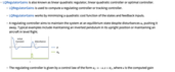
- A regulating controller aims to maintain the system at an equilibrium state despite disturbances
 pushing it away. Typical examples include maintaining an inverted pendulum in its upright position or maintaining an aircraft in level flight.
 - The regulating controller is given by a control law of the form
 , where
  is the computed gain matrix.
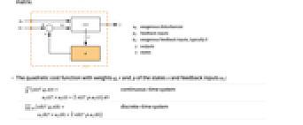
 - The quadratic cost function with weights q, r and p of the states x and feedback inputs uf:
-

continuous-time system 
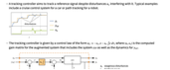
discrete-time system - A tracking controller aims to track a reference signal despite disturbances
 interfering with it. Typical examples include a cruise control system for a car or path tracking for a robot.
 - The tracking controller is given by a control law of the form
 , where
  is the computed gain matrix for the augmented system that includes the system sys as well as the dynamics for
  .
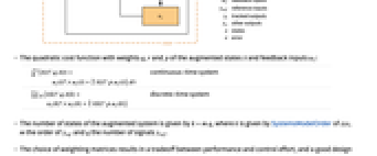
. - The quadratic cost function with weights q, r and p of the augmented states
 and feedback inputs uf:
 -

continuous-time system 
discrete-time system - The number of states of the augmented system is given by
 , where
  is given by SystemsModelOrder of sys,
  the order of yref and
  the number of signals yref.
 - The choice of weighting matrices results in a tradeoff between performance and control effort, and a good design is arrived at iteratively. Their starting values can be diagonal matrices with entries
![TemplateBox[{{1, /, z}, i, 2}, Subsuperscript]](Files/LQRegulatorGains.en/21.png "TemplateBox[{{1, /, z}, i, 2}, Subsuperscript]") , where zi is the maximum admissible absolute value of the corresponding xi or ui.
, where zi is the maximum admissible absolute value of the corresponding xi or ui. - The weights wts can have the following forms:
-
{q,r} cost function with no cross-coupling {q,r,p} cost function with cross-coupling matrix p - LQ design works for linear systems as specified by StateSpaceModel:
-

continuous-time system 
discrete-time system - The resulting feedback gain matrix
 is then computed from algebraic Riccati equations:
 -
![kappa=TemplateBox[{r}, Inverse].(b_f.x_r+p)](Files/LQRegulatorGains.en/25.png "kappa=TemplateBox[{r}, Inverse].(b_f.x_r+p)")
continuous-time system and  is the solution to the continuous-time algebraic Riccati equation
 ![a.x_r+x_r.a-(x_r.b_f+p).TemplateBox[{r}, Inverse].(b_f.x_r+p)+q=0](Files/LQRegulatorGains.en/27.png "a.x_r+x_r.a-(x_r.b_f+p).TemplateBox[{r}, Inverse].(b_f.x_r+p)+q=0")
![kappa=TemplateBox[{{(, {{{{b, _, f}, }, ., {x, _, r}, ., {b, _, f}}, +, r}, )}}, Inverse].(b_f.x_r.a+p)](Files/LQRegulatorGains.en/28.png "kappa=TemplateBox[{{(, {{{{b, _, f}, }, ., {x, _, r}, ., {b, _, f}}, +, r}, )}}, Inverse].(b_f.x_r.a+p)")
discrete-time system and  is the solution to the discrete-time algebraic Riccati equation
 ![a.x_r.a-x_r-(a.x_r.b_f+p)TemplateBox[{{., {(, {{{{b, _, f}, }, ., {x, _, r}, ., {b, _, f}}, +, r}, )}}}, Inverse].(b_f.x_r.a+p)+q=0](Files/LQRegulatorGains.en/30.png "a.x_r.a-x_r-(a.x_r.b_f+p)TemplateBox[{{., {(, {{{{b, _, f}, }, ., {x, _, r}, ., {b, _, f}}, +, r}, )}}}, Inverse].(b_f.x_r.a+p)+q=0") .
. - The submatrix bf is columns of b corresponding to the feedback inputs uf.
- The system specification sspec is the system sys together with the uf, yt and yref specifications.
- The system specification sspec can have the following forms:
-
StateSpaceModel[…] linear control input and linear state AffineStateSpaceModel[…] linear control input and nonlinear state NonlinearStateSpaceModel[…] nonlinear control input and nonlinear state SystemModel[…] general system model <…> detailed system specification given as an Association - The detailed system specification can have the following keys:
-
"InputModel" sys any one of the models "FeedbackInputs" All the feedback inputs uf "TrackedOutputs" None the tracked outpus yt "TrackedSignal" Automatic the dynamics of yref - The feedback inputs can have the following forms:
-
{num1,…,numn} numbered inputs numi used by StateSpaceModel, AffineStateSpaceModel and NonlinearStateSpaceModel {name1,…,namen} named inputs namei used by SystemModel All uses all inputs - For nonlinear systems such as AffineStateSpaceModel, NonlinearStateSpaceModel and SystemModel, the system will be linearized around its stored operating point.
- LQRegulatorGains[…,"Data"] returns a SystemsModelControllerData object cd that can be used to extract additional properties using the form cd["prop"].
- LQRegulatorGains[…,"prop"] can be used to directly give the value of cd["prop"].
- Possible values for properties "prop" include:
-
"ClosedLoopPoles" poles of the linearized "ClosedLoopSystem" "ClosedLoopSystem" system csys {"ClosedLoopSystem", cspec} detailed control over the form of the closed-loop system "ControllerModel" model cm "Design" type of controller design "DesignModel" model used for the design "FeedbackGains" gain matrix κ or its equivalent "FeedbackGainsModel" model gm or {gm1,gm2} "FeedbackInputs" inputs uf of sys used for feedback "InputModel" input model sys "InputCount" number of inputs u of sys "OpenLoopPoles" poles of "DesignModel" "OutputCount" number of outputs y of sys "SamplingPeriod" sampling period of sys "StateCount" number of states x of sys "TrackedOutputs" outputs yt of sys that are tracked - Possible keys for cspec include:
-
"InputModel" input model in csys "Merge" whether to merge csys "ModelName" name of csys - The diagram of the regulator layout.
- The diagram of the tracker layout.
Examples
open allclose allBasic Examples (3)
The optimal feedback gains for a system specification sspec with a feedback uf and exogenous input ue:
The optimal gains for a specified set of control weights q and r:
The feedback gains for a nonlinear system for a specified set of control weights wts:
The gains have an offset because of the nonzero operating points:
The gains of the approximate linear system do not have the offset:
The controller data object for a specified set of weights wts:
Scope (33)
Basic Uses (9)
Compute the state feedback gain of a system with equal weighting for the state and input:
Compute the gain for an unstable system:
The gain stabilizes the unstable system:
Compute the state feedback gains for a multiple-state system:
The dimensions of the result correspond to the number of inputs and the system's order:
Compute the gains for a system with 3 states and 2 inputs:
Reverse the weights of the feedback inputs:
Typically, the feedback input with the bigger weight has the smaller norm:
Compute the gains when the cost function contains cross-coupling of the states and feedback inputs:
Choose the feedback inputs for multiple-input systems:
Compute the set of feedback gains for a stabilizable but uncontrollable system:
Compute the gains for a nonlinear system:
The controller is returned as a vector and takes operating points into consideration:
The controller for the approximate linear system:
Compute the gains when the cost is given as a quadratic function of states and feedback inputs:
Plant Models (6)
Properties (10)
LQRegulatorGains returns the feedback gains by default:
In general, the feedback is affine in the states:
It is of the form κ.x+λ, where κ and λ are constants:
The systems model of the feedback gains:
An affine systems model of the feedback gains:
The poles of the linearized closed-loop system:
Increasing the weight of the states makes the system more stable:
Increasing the weight of the feedback inputs makes the system less stable:
The model used to compute the feedback gains:
The feedback gains structure is different if the design model is directly specified in the input:
Properties related to the input model:
Get the controller data object:
Tracking (5)
The closed-loop system tracks the reference signal ![]() :
:
Design a tracking controller for a discrete-time system:
The closed-loop system tracks the reference signal ![]() :
:
The closed-loop system tracks two different reference signals:
Compute the controller effort:
Track a desired reference signal:
The reference signal is of order 2:
Design a controller to track one output of a first-order system:
Closed-Loop System (3)
Assemble the closed-loop system for a nonlinear plant model:
The closed-loop system with a linearized model:
Compare the response of the two systems:
Assemble the merged closed loop of a plant with one disturbance and one feedback input:
The unmerged closed-loop system:
When merged, it gives the same result as before:
Explicitly specify the merged closed-loop system:
Create a closed-loop system with a desired name:
The closed-loop system has the specified name:
The name can be directly used to specify the closed-loop model in other functions:
Applications (11)
Mechanical Systems (2)
The system modeled as an inverted pendulum:
The Segway tips over if perturbed:
Design a balancing controller:
Obtain the closed-loop system:
Compute the response of the balanced system to a nonzero initial condition:
Tune the damping of a car suspension:
The response of the suspension to a bump on the road is very pronounced:
Set the active damping force as the only feedback input:
Design an optimal controller to dampen the oscillations in the response:
Electromechanical Systems (4)
Levitate a ball about an equilibrium point:
A model of the system with equilibrium point ![]() :
:
Without feedback, the ball falls down:
Set the input voltage as the sole feedback input:
Design a feedback controller to levitate the ball:
Obtain the closed-loop system:
The ball is levitated to the equilibrium point ![]() :
:
The velocity of the ball and current of the electromagnet:
Regulate the angular position of a motor:
The angular position of the motor is unregulated to a torque disturbance:
Design a controller to reject the disturbance:
Regulate a ball and beam system:
If the beam is not horizontal, the ball rolls away:
Design a state feedback controller to return the ball to its original position:
Obtain the closed-loop system:
The controlled system returns the ball to its original position:
Design an analog gauge that tracks a sinusoid:
The sinusoidal signal to track:
Set the current as the only input, and the sinusoidal signal as the tracked signal:
Design a controller that tracks the sinusoidal signal:
Aerospace Systems (2)
Improve the handling qualities of an aircraft:
The open-loop response to a disturbance in the pitch angle takes about ![]() seconds to stabilize:
seconds to stabilize:
Compute a set of regulator and estimator gains:
Assemble an estimator-regulator:
The handling response is improved:
Stabilize the longitudinal dynamics of a helicopter:
A model of the helicopter's dynamics:
There are three poles on the right-hand side of the ![]() plane:
plane:
Hence its unstable response to a change in the forward pitch angle:
Design an optimal controller to stabilize the pitch angle:
Obtain the closed-loop system:
The closed-loop system is stable:
Electrical Systems (1)
The open-loop pole locations reveal the system is stable:
However, the system's response has near resonance at frequencies close to 1000 rad/s:
Design a set of controllers with increasing gains to tune the response:
The closed-loop pole locations:
The response is better damped close to 1000 rad/s as the weight is increased:
Chemical Systems (1)
Nautical Systems (1)
Regulate the heading of a boat:
A state-space model of the system:
The poles indicate the system is marginally stable:
The heading angle deviates from the equilibrium for nonzero initial conditions:
Design a feedback controller to regulate the boat's heading:
Properties & Relations (24)
The optimal gains are computed for negative feedback:
The closed-loop poles with negative feedback ![]() :
:
They are the same as the computed poles:
The closed-loop system is obtained using state feedback:
Obtain it directly as a property:
For a nonlinear system, the gains are affine and of the form ![]() :
:
The gains of the linearized system are linear of the form ![]() :
:
The affine gains are obtained by solving ![]() :
:
An LQR design has guaranteed gain and phase margins:
The phase margin is at least ![]() :
:
This is because the Nyquist plot always lies outside the unit circle centered at ![]() :
:
A controllable standard StateSpaceModel can be completely controlled using state feedback:
The closed- and open-loop poles:
A controllable nonsingular descriptor StateSpaceModel can also be completely controlled:
The closed- and open-loop poles:
Only a subsystem of an uncontrollable standard StateSpaceModel can be controlled:
The eigenvalue ![]() is controllable and
is controllable and ![]() is not:
is not:
The uncontrollable eigenvalue ![]() is not affected:
is not affected:
Only the controllable slow subsystem of a singular descriptor system can be controlled:
The dimension of the slow subsystem:
The gain corresponding to the fast subsystem is ![]() :
:
The pole of the slow subsystem is moved but the pole at ![]() of the fast subsystem is unchanged:
of the fast subsystem is unchanged:
The complete system is uncontrollable and is of order less than the number of states:
A singular descriptor system with an uncontrollable slow subsystem is completely uncontrollable:
The dimension of the slow subsystem:
None of the poles are changed:
A stabilizable system can be stabilized using state feedback:
One of the eigenvalues is unstable:
The system is uncontrollable but stabilizable:
LQRegulatorGains can compute the stabilizing gains for the system:
The state feedback brings the unstable eigenvalue to the left half-plane and leaves the other unchanged:
For continuous-time systems, the gains are computed using RiccatiSolve:
LQRegulatorGains gives the same result:
For discrete-time systems, the gains are computed using DiscreteRiccatiSolve:
LQRegulatorGains gives the same result:
A larger state weight results in a faster state response:
A larger control weight results in a slower state response:
For a stable system, a larger control weight causes closed-loop poles to approach open-loop poles:
The distance of the closed-loop poles from the open-loop poles:
For an unstable system, a larger control weight causes closed-loop poles to approach the negative of open-loop poles:
The distance of the closed-loop poles from the negative of the open-loop poles:
LQRegulatorGains and FullInformationOutputRegulator give the same results:
LQRegulatorGains and StateFeedbackGains yield the same results for a single-input system:
StateFeedbackGains with the closed-loop poles of the LQRegulatorGains design:
LQRegulatorGains gives the same gains:
An estimator-regulator is assembled using LQRegulatorGains and EstimatorGains:
Compute the regulator and estimator gains:
Obtain the estimator-regulator using the computed gains:
The optimal cost ![]() is a Lyapunov function:
is a Lyapunov function:
Its Hessian is positive definite:
The state trajectory projected on the optimal cost surface asymptotically approaches the origin:
The optimal cost satisfies the infinite horizon Hamilton–Jacobi–Bellman (HJB) equation:
The optimal co-state trajectory:
The optimal input is a extremum:
The solutions of the HJB equation:
The solution is the optimal cost:
The input based on the HJB solution is the computed optimal input:
The costate based on the HJB solution is the computed optimal costate:
The optimal solution satisfies ![]() , where
, where ![]() is the Hamiltonian:
is the Hamiltonian:
The optimal solutions of the state:
The optimal input minimizes the Hamiltonian, thus satisfying ![]() :
:
State feedback does not alter the input-blocking properties of a system:
The closed-loop system for a specific set of weights:
Both the open- and closed-loop systems block the input Sin[2t]:
The weight ![]() that minimizes
that minimizes ![]() ρ c.c x(t)2+u(t)2t results in a closed-loop system with poles given by the symmetric root locus:
ρ c.c x(t)2+u(t)2t results in a closed-loop system with poles given by the symmetric root locus:
The symmetric root locus plot:
The poles on the plot for the parameter value ![]() are those of the closed-loop system:
are those of the closed-loop system:
Possible Issues (4)
If ![]() has unobservable modes on the imaginary axis, there is no continuous-time solution:
has unobservable modes on the imaginary axis, there is no continuous-time solution:
The zero eigenvalue is unobservable:
If ![]() has unobservable modes on the unit circle, there is no discrete-time solution:
has unobservable modes on the unit circle, there is no discrete-time solution:
The eigenvalue 1 is unobservable:
The gain computations fail if the control weighting matrix is not positive definite:
Use a positive-definite control weighting matrix:
It is not possible to compute an optimal regulator for a system that is not stabilizable:
Text
Wolfram Research (2010), LQRegulatorGains, Wolfram Language function, https://reference.wolfram.com/language/ref/LQRegulatorGains.html (updated 2021).
CMS
Wolfram Language. 2010. "LQRegulatorGains." Wolfram Language & System Documentation Center. Wolfram Research. Last Modified 2021. https://reference.wolfram.com/language/ref/LQRegulatorGains.html.
APA
Wolfram Language. (2010). LQRegulatorGains. Wolfram Language & System Documentation Center. Retrieved from https://reference.wolfram.com/language/ref/LQRegulatorGains.html