

GreenFunction
GreenFunction[{ℒ[u[x]],ℬ[u[x]]},u,{x,xmin,xmax},y]
gives a Green's function for the linear differential operator ℒ with boundary conditions ℬ in the range xmin to xmax.
GreenFunction[{ℒ[u[x1,x2,…]],ℬ[u[x1,x2,…]]},u,{x1,x2,…}∈Ω,{y1,y2,…}]
gives a Green's function for the linear partial differential operator ℒ over the region Ω.
GreenFunction[{ℒ[u[x,t]],ℬ[u[x,t]]},u,{x,xmin,xmax},t,{y,τ}]
gives a Green's function for the linear time-dependent operator ℒ in the range xmin to xmax.
GreenFunction[{ℒ[u[x1,…,t]],ℬ[u[x1,…,t]]},u,{x1,…}∈Ω,t,{y1,…,τ}]
gives a Green's function for the linear time-dependent operator ℒ over the region Ω.
Details and Options
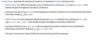
- GreenFunction represents the response of a system to an impulsive DiracDelta driving function.
- GreenFunction for a differential operator
 is defined to be a solution
  of
of ![L(G(x;y))=TemplateBox[{{x, -, y}}, DiracDeltaSeq]](Files/GreenFunction.en/3.png "L(G(x;y))=TemplateBox[{{x, -, y}}, DiracDeltaSeq]") that satisfies the given homogeneous boundary conditions
that satisfies the given homogeneous boundary conditions  .
. - A particular solution of
 with homogeneous boundary conditions
  can be obtained by performing a convolution integral
  .
. - GreenFunction for a time-dependent differential operator
 is defined to be a solution
  of
of ![L(G(x,t;y,tau))=TemplateBox[{{x, -, y}}, DiracDeltaSeq]TemplateBox[{{t, -, tau}}, DiracDeltaSeq]](Files/GreenFunction.en/10.png "L(G(x,t;y,tau))=TemplateBox[{{x, -, y}}, DiracDeltaSeq]TemplateBox[{{t, -, tau}}, DiracDeltaSeq]") that satisfies the given homogeneous boundary conditions
that satisfies the given homogeneous boundary conditions  .
. - A particular solution of
 with homogeneous boundary conditions
  can be obtained by performing a convolution integral
  .
. - The Green's functions for classical PDEs have characteristic geometrical properties:
 is given as an expression in
  and
and  if the dependent variable is of the form
  , and as a pure function with formal parameters
  and
and  if the dependent variable is of the form
  instead of
  . »
. »- The region Ω can be anything for which RegionQ[Ω] is True.
- All the necessary initial and boundary conditions for ODEs must be specified in
 .
. - Boundary conditions for PDEs must be specified using DirichletCondition or NeumannValue in
 .
. - Assumptions on parameters may be specified using the Assumptions option.
Examples
open all close allBasic Examples (2)
Scope (22)
Basic Uses (2)
Compute the Green's function for an ordinary differential operator:
Obtain a pure function in the result by using u instead of u[x] in the second argument:
Compute the Green's function for a partial differential operator:
Obtain a pure function in the result by using u instead of u[x,t] in the second argument:
Ordinary Differential Equations (4)
Wave Equation (4)
Green's function for the wave operator on the real line:
Green's function for the wave operator with a Dirichlet condition on a half-line:
Green's function for the wave operator with a Neumann condition on a half-line:
Green's function for the wave operator with a Dirichlet condition on an interval:
Heat Equation (5)
Green's function for the heat operator on the real line:
Green's function for the heat operator with a Dirichlet condition on a half-line:
Green's function for the heat operator with a Dirichlet condition on an interval:
Green's function for the heat operator with a Neumann condition on an interval:
Laplace Equation (4)
Options (1)
Assumptions (1)
Specify Assumptions on parameters in GreenFunction:
Applications (9)
Ordinary Differential Equations (4)
Solve an initial value problem for an inhomogeneous differential equation using GreenFunction:
Perform a convolution of the Green's function with the forcing function:
Compare with the result given by DSolveValue:
Solve a Dirichlet problem for an inhomogeneous differential equation using GreenFunction:
Perform a convolution of the Green's function with the forcing function:
Compare with the result given by DSolveValue:
Solve a Neumann problem for an inhomogeneous differential equation using GreenFunction:
Perform a convolution of the Green's function with the forcing function:
Compare with the result given by DSolveValue:
Solve a Robin problem for an inhomogeneous differential equation using GreenFunction:
Perform a convolution of the Green's function with the forcing function:
Compare with the result given by DSolveValue:
Partial Differential Equations (2)
Solve the inhomogeneous wave equation using GreenFunction:
Define the inhomogeneous term:
Solve the inhomogeneous equation using ![]() :
:
Compare with the solution given by DSolveValue:
Solve an initial value problem for the heat equation using GreenFunction:
Solve the initial value problem using ![]() :
:
Compare with the solution given by DSolveValue:
Physics and Engineering (3)
Compute the current i[t] in a circuit with a voltage source v[t] that is connected to a resistor R and an inductor L. The operator for this circuit is given by:
Find the current for a given voltage source:
Compute the displacement u[x] for a string of length p and tension T that is fixed at the two ends and is subjected to a force per unit length of f[x]. The operator for the displacement is given by:
Find the displacement for a given force:
The impulse response of a continuous linear time-invariant system can be found by using the Green's function for the system with homogeneous initial conditions. Compute the impulse response for the system defined by:
Green's function for the system with homogeneous initial conditions:
Properties & Relations (2)
Compute a Green's function for a differential equation:
Obtain the same result using DSolve:
GreenFunction is related to OutputResponse and TransferFunctionModel:
Text
Wolfram Research (2016), GreenFunction, Wolfram Language function, https://reference.wolfram.com/language/ref/GreenFunction.html.
CMS
Wolfram Language. 2016. "GreenFunction." Wolfram Language & System Documentation Center. Wolfram Research. https://reference.wolfram.com/language/ref/GreenFunction.html.
APA
Wolfram Language. (2016). GreenFunction. Wolfram Language & System Documentation Center. Retrieved from https://reference.wolfram.com/language/ref/GreenFunction.html