

ParametricNDSolveValue
ParametricNDSolveValue[eqns,expr,{x,xmin,xmax},pars]
gives the value of expr with functions determined by a numerical solution to the ordinary differential equations eqns with the independent variable x in the range xmin to xmax with parameters pars.
ParametricNDSolveValue[eqns,expr,{x,xmin,xmax},{y,ymin,ymax},pars]
solves the partial differential equations eqns over a rectangular region.
ParametricNDSolveValue[eqns,expr,{x,y}∈Ω,pars]
solves the partial differential equations eqns over the region Ω.
ParametricNDSolveValue[eqns,expr,{t,tmin,tmax},{x,y}∈Ω,pars]
solves the time-dependent partial differential equations eqns over the region Ω.
Details and Options
- ParametricNDSolveValue gives results in terms of ParametricFunction objects.
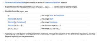
- A specification for the parameters pars of {pspec1,pspec2,…} can be used to specify ranges.
- Possible forms for pspeci are:
-
p p has range Reals or Complexes Element[p,Reals] p has range Reals Element[p,Complexes] p has range Complexes Element[p,{v1,…}] p has discrete range {v1,…} {p,pmin,pmax} p has range 
- Typically expr will depend on the parameters indirectly, through the solution of the differential equations, but may depend explicitly on the parameters.
- Derivatives of the resulting ParametricFunction object with respect to the parameters are computed using a combination of symbolic and numerical sensitivity methods when possible.
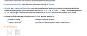
- ParametricNDSolveValue takes the same options and settings as NDSolve.
- NDSolve and ParametricNDSolveValue typically solve differential equations by going through several different stages, depending on the type of equations. With Method->{s1->m1,s2->m2,…}, stage si is handled by method mi. The actual stages used and their order are determined by NDSolve, based on the problem to be solved.
- Possible solution stages are the same as for NDSolve, with the addition of:
-
"ParametricCaching" caching of computed solutions "ParametricSensitivity" computation of derivatives with respect to parameters
List of all options

Examples
open all close allBasic Examples (3)
Get a parametric function of the parameter a for the value of y:
Evaluating with a numerical value of a gives an approximate function solution for y:
Plot the solutions for several different values of the parameter:
Get a function of the parameter a that gives the value of the function f at ![]() :
:
This plots the value as a function of the parameter a:
Use the function with FindRoot to find a root:
Show the sensitivity of the solution of a differential equation to parameters:
Scope (6)
Parameter Dependence (4)
ParametricNDSolveValue returns a ParametricFunction object:
Plot solutions for values of ![]() ranging from
ranging from ![]() to
to ![]() :
:
Initial conditions can be specified as parameters:
Plot solutions with ![]() with
with ![]() for values of
for values of ![]() ranging from
ranging from ![]() to
to ![]() :
:
Plot solutions with ![]() with
with ![]() for values of
for values of ![]() ranging from
ranging from ![]() to
to ![]() :
:
Return a function of the solution ![]() :
:
Differential equation coefficients and boundary conditions can be specified as parameters:
Plot solutions with ![]() for values of
for values of ![]() ranging from
ranging from ![]() to
to ![]() and with
and with ![]() and
and ![]() :
:
Parameter Sensitivity (2)
Solve the classical harmonic oscillator with parametric amplitude a:
Plot the solution for ![]() and several nearby values of
and several nearby values of ![]() :
:
The sensitivity of ![]() with respect to
with respect to ![]() is by definition
is by definition ![]() . Plot the sensitivity at
. Plot the sensitivity at ![]() :
:
Plot the sensitivity ![]() as a band around the solution
as a band around the solution ![]() for
for ![]() :
:
Sensitivity analysis of a differential equation with multiple parameters:
Plot the sensitivity with respect to the initial condition ![]() at
at ![]() ,
, ![]() :
:
Plot the sensitivity with respect to the initial condition ![]() at
at ![]() ,
, ![]() :
:
Generalizations & Extensions (2)
Solve ![]() ,
, ![]() for various values of WorkingPrecision and plot the error:
for various values of WorkingPrecision and plot the error:
Consider finding a solution to a highly nonlinear problem that NDSolveValue cannot solve directly. Set up a boundary condition, a region and the equation that depends on a parameter ![]() :
:
NDSolveValue cannot find a solution:
Set up an initial seeding function:
Create a ParametricNDSolveValue function based on the parameter ![]() :
:
Reset the seeding to use the solution from ![]() :
:
Options (2)
Method (2)
ParametricCaching (1)
Applications (14)
Parameter Sweeps (7)
Simulate bouncing balls being dropped from various heights:
Find an initial value ![]() for which the solution
for which the solution ![]() of a differential equation will have
of a differential equation will have ![]() :
:
Compare to nearby values of the parameter s:
Find several solutions to the boundary value problem ![]() ,
, ![]() ,
, ![]() . First consider several possible values for
. First consider several possible values for ![]() :
:
Run a parameter sweep to determine nontrivial solution values of ![]() :
:
Using approximate initial values from the graph above:
Plot the solutions that were found:
Find all eigenvalues ![]() and eigenfunctions
and eigenfunctions ![]() for the classical harmonic oscillator
for the classical harmonic oscillator ![]() with
with ![]() . Start by exploring the possible parameter values:
. Start by exploring the possible parameter values:
Find the first three eigenfunctions of the quantum harmonic oscillator ![]() ,
, ![]() ,
, ![]() . Start by plotting solutions of
. Start by plotting solutions of ![]() for
for ![]() :
:
The roots are the approximate eigenvalues. Find the first three:
Plot the approximate eigenfunctions together with solutions for nearby ![]() :
:
These only differ from the exact eigenfunctions, the Hermite functions, by scaling factors:
Find the value of ![]() for which the solution of
for which the solution of ![]() ,
, ![]() has minimal arc length from
has minimal arc length from ![]() to
to ![]() . Begin by plotting the solutions for values of
. Begin by plotting the solutions for values of ![]() ranging from 0 to 1:
ranging from 0 to 1:
Plot ![]() versus the arc length of the solution:
versus the arc length of the solution:
The minimum arc length solution for ![]() seems to occur at
seems to occur at ![]() :
:
Find the local minimum, which appears near ![]() :
:
Plot the corresponding solution of (locally) minimal arc length together with some nearby solutions:
Simulate the response of an RLC circuit to a step in the voltage v1 at time ![]() :
:
Parameter Sensitivities (5)
Perturb a parameter in a differential equation and view several of the resulting perturbed solutions:
A plot of the solution with its sensitivity band is qualitatively similar:
Simulate an inverted pendulum stabilized by a base oscillating with frequency ω and amplitude a:
With ![]() ,
, ![]() the pendulum is stabilized near an inverted position
the pendulum is stabilized near an inverted position ![]() , but the sensitivity increases:
, but the sensitivity increases:
Find the sensitivity of the Lorenz equations to a parameter:
Parametric dependence of the heat equation ![]() ,
, ![]() :
:
Plot the corresponding sensitivity bands:
Indicate sensitivity to a and c by changing the color of the solution surface:
Parametric dependence of the wave equation ![]() ,
, ![]() :
:
Plot the corresponding sensitivity bands:
Indicate sensitivity to a and c by changing the color of the solution surface:
Parameter Fitting (2)
Sample the solution of a differential equation and add noise:
Fit a trigonometric model to the noisy data:
A quadratic model is a better fit:
Find the parameters that make the solution of a differential equation the best fit to data:
Convert data to kelvins and find initial and final (ambient) temperatures:
Find solutions to Newton's law of cooling depending on parameters k1 and k2:
Fit the parameters in the differential equation to the given data:
Properties & Relations (3)
Use NDSolveValue to solve differential equations with parameters:
For a given parameter value, each function call takes roughly the same amount of time:
ParametricNDSolve caches the solution and subsequently reuses the cached solution values:
DSolve can solve some differential equations with parameters in closed form:
Use ParametricNDSolveValue to solve the example numerically:
The sensitivity is the same from both paths:
Use SystemModelParametricSimulate to simulate larger hierarchical system models:
Simulate with two sets of resistor and spring damper parameters:
Text
Wolfram Research (2012), ParametricNDSolveValue, Wolfram Language function, https://reference.wolfram.com/language/ref/ParametricNDSolveValue.html (updated 2014).
CMS
Wolfram Language. 2012. "ParametricNDSolveValue." Wolfram Language & System Documentation Center. Wolfram Research. Last Modified 2014. https://reference.wolfram.com/language/ref/ParametricNDSolveValue.html.
APA
Wolfram Language. (2012). ParametricNDSolveValue. Wolfram Language & System Documentation Center. Retrieved from https://reference.wolfram.com/language/ref/ParametricNDSolveValue.html