TimeSeriesModelFit[data]
constructs a time series model for data from an automatically selected model family.
TimeSeriesModelFit[data,mspec]
constructs a time series model for data from a model family specified by mspec.


TimeSeriesModelFit
TimeSeriesModelFit[data]
constructs a time series model for data from an automatically selected model family.
TimeSeriesModelFit[data,mspec]
constructs a time series model for data from a model family specified by mspec.
Details and Options
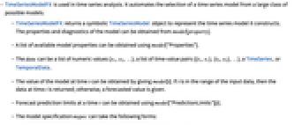
- TimeSeriesModelFit is used in time series analysis. It automates the selection of a time series model from a large class of possible models.
- TimeSeriesModelFit returns a symbolic TimeSeriesModel object to represent the time series model it constructs. The properties and diagnostics of the model can be obtained from model[property].
- A list of available model properties can be obtained using model["Properties"].
- The data can be a list of numeric values {x1,x2,…}, a list of time-value pairs {{t1,x1},{t2,x2},…}, a TimeSeries, or TemporalData.
- The value of the model at time t can be obtained by giving model[t]. If t is in the range of the input data, then the data at time t is returned; otherwise, a forecasted value is given.
- Forecast prediction limits at a time t can be obtained using model["PredictionLimits"][t].
- The model specification mspec can take the following forms:
-
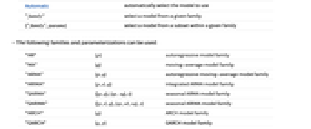
Automatic automatically select the model to use "family" select a model from a given family {"family",params} select a model from a subset within a given family - The following families and parameterizations can be used:
-
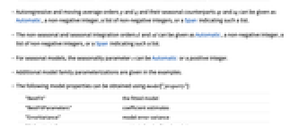
"AR" {p} autoregressive model family "MA" {q} moving-average model family "ARMA" {p,q} autoregressive moving-average model family "ARIMA" {p,d,q} integrated ARMA model family "SARMA" {{p,q},{sp,sq},s} seasonal ARMA model family "SARIMA" {{p,d,q},{sp,sd,sq},s} seasonal ARIMA model family "ARCH" {q} ARCH model family "GARCH" {q,p} GARCH model family - Autoregressive and moving-average orders p and q and their seasonal counterparts sp and sq can be given as Automatic, a non-negative integer, a list of non-negative integers, or a Span indicating such a list.
- The non-seasonal and seasonal integration orders d and sd can be given as Automatic, a non-negative integer, a list of non-negative integers, or a Span indicating such a list.
- For seasonal models, the seasonality parameter s can be Automatic or a positive integer.
- Additional model family parameterizations are given in the examples.
- The following model properties can be obtained using model["property"]:
-
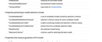
"BestFit" the fitted model "BestFitParameters" coefficient estimates "ErrorVariance" model error variance "FitResiduals" residuals for the fitted model "StandardizedResiduals" standardized model residuals "TemporalData" input data as TemporalData - Properties pertaining to model selection include:
-
"CandidateModels" a set of candidate models sorted by selection criterion "CandidateModelSelectionValues" selection criterion values for each candidate model "CandidateSelectionTable" a table containing models and selection criterion values "CandidateSelectionTableEntries" entries from the candidate selection table "ModelFamily" the selected model family "SelectionCriterion" criterion used for selecting the best model - Properties that measure goodness of fit include:
-
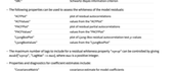
"AIC" Akaike information criterion "AICc" finite sample corrected AIC "BIC" Bayesian information criterion "SBC" Schwartz–Bayes information criterion - The following properties can be used to assess the whiteness of the model residuals:
-
"ACFPlot" plot of residual autocorrelations "ACFValues" values from the "ACFPlot" "PACFPlot" plot of residual partial autocorrelations "PACFValues" values from the "PACFPlot" "LjungBoxPlot" plot of Ljung–Box residual autocorrelation test  -values
"LjungBoxValues" values from the "LjungBoxPlot" - The maximum number of lags to include for a residual whiteness property "wprop" can be controlled by giving model["wprop","LagMax"->max], where max is a positive integer.
- Properties and diagnostics for coefficient estimates include:
-
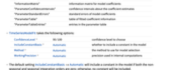
"CovarianceMatrix" covariance estimate for model coefficients "InformationMatrix" information matrix for model coefficients "ParameterConfidenceIntervals" confidence intervals about the coefficient estimates "ParameterStandardErrors" standard errors of model coefficients "ParameterTable" table of fitted coefficient information "ParameterTableEntries" entries in the parameter table - TimeSeriesModelFit takes the following options:
-
ConfidenceLevel 95/100 confidence level to choose » IncludeConstantBasis Automatic whether to include a constant in the model » Method Automatic the method to use for model selection » WorkingPrecision Automatic precision used in internal computations » - The default setting IncludeConstantBasis->Automatic will include a constant in the model if both the non-seasonal and seasonal integration orders are zero; otherwise, no constant will be included.
- The method m in Method->m can be either "Stepwise" or "GridSearch". For stepwise selection, Automatic parameter orders are incrementally changed until a model with an optimal selection criterion is found. Using a grid search exhaustively tries all models over a specified grid.
- The best model is selected according to a selection criterion crit, which can be set in Method->{m,"SelectionCriterion"->crit}. Some examples of valid selection criteria include "AIC" (default), "AICc", "SBC", and "BIC".
Examples
open all close allBasic Examples (1)
Scope (22)
Basic Uses (5)
Automatically fit a model to a time series:
The model selected for the data:
Create a forecast using some monthly temperature data:
The monthly temperature data and a 24-month forecast:
Forecast the average temperature for June 1, 2014:
A 95% confidence interval about the forecast:
Fit a particular model to a time series:
Fit a "GARCH"(1,1) model to the data:
The model and parameter estimates:
Fit a time series model to a 100-business-day time series:
Simulate the next 30 business days 50 times:
Use the original data to simulate future observations with TimeSeriesModel:
Use the best-fit process to simulate 10 future observations:
No information about time stamps or initial values is passed to RandomFunction:
Simulate using TimeSeriesModel to use information given by the original data:
Model Specification (6)
Automatically select a model for a time series:
Equivalently, specify Automatic:
Find a model in a particular family:
Search the autoregressive family of models:
Select the best model from an explicit set of candidates:
Search the ARMA family with orders ![]() and
and ![]() from 0 to 2:
from 0 to 2:
Fit a model with fixed orders:
Fit an "ARIMA"(2,1,3) model to the data:
Fix the integration order and search for the autoregressive and moving average orders:
Parameterizations for the ARIMA family of models:
Automatically detect the orders ![]() ,
, ![]() , and
, and ![]() :
:
Alternatively, use Automatic for all parameter orders:
Equivalent ways to fix the integration order ![]() while leaving
while leaving ![]() and
and ![]() Automatic:
Automatic:
Equivalent ways to fix ![]() and
and ![]() while leaving the integration order
while leaving the integration order ![]() Automatic:
Automatic:
Parameterizations for the SARIMA family of models:
Automatically detect ![]() ,
, ![]() ,
, ![]() ,
, ![]() ,
, ![]() ,
, ![]() , and
, and ![]() :
:
Alternatively, use Automatic for all parameter orders:
Equivalent ways to fix the seasonality parameter ![]() while leaving all others Automatic:
while leaving all others Automatic:
Equivalent ways to fix the seasonality ![]() and integration orders
and integration orders ![]() and
and ![]() :
:
Model Properties (11)
Obtain a list of available properties:
Extract the best-fitting process:
Equivalently, use Normal:
Show some fit criteria for the selected model:
The criterion that was used to choose the best model:
Report the top models that were fitted to the data:
Obtain a list of candidate models fitted to the data:
Check whether fit residuals are autocorrelated:
There is a significant spike at lag 3:
Adding a moving-average component removes the autocorrelation at lag 3:
Check whether the partial correlation function for the fit residuals is zero:
There is a significant spike at lag 3:
Adding a moving-average component removes the partial correlation at lag 3:
Test model residuals for autocorrelation:
There are significant spikes at lags 3 and 4:
Adding a moving-average component removes the significant autocorrelations:
Obtain values used in residual whiteness diagnostic plots:
The first 5 autocorrelation values and 95% confidence region used in the "ACFPlot":
The first 5 partial autocorrelation values and 95% confidence region used in the "PACFPlot":
The Ljung–Box ![]() -values for lags 1 to 12 and the critical value used in the plot:
-values for lags 1 to 12 and the critical value used in the plot:
Report the values and significance of model parameters:
The value entries from the table:
Obtain parameter standard errors from the parameter covariance matrix:
Options (9)
ConfidenceLevel (2)
Set the confidence level to use for prediction limits:
The confidence level can be changed after fitting:
The ConfidenceLevel setting affects thresholds for feature detection:
IncludeConstantBasis (1)
Method (5)
By default, parameter orders are selected using a stepwise search:
Use different selection criteria to pick the best model:
Set the maximum number of candidate models to keep for reporting:
Retain a maximum of 15 models:
Keep all models that were fitted:
By default, a maximum of 10 models are kept:
Set the maximum allowable autoregressive and moving-average orders:
The maximum orders limit the number of models that can be fitted:
The stepwise method fits models within "MaxStepSize" orders of the current best model:
By default, the maximum order step is set to 1:
Increasing the step size can improve quality but may increase search time:
WorkingPrecision (1)
Use WorkingPrecision to obtain higher-precision estimates:
Applications (8)
Local Temperature (1)
Airline Passengers (2)
The following data contains the monthly total number of US international airline passengers (in thousands) from January 1949 to December 1960:
Split the data at January 1958:
Fit a time series model to the airline passenger data before 1958:
Compare the forecasted and actual number of airline passengers for June of 1959:
The forecast from 1958 to 1961 compared to the actual data:
Simulate airline passenger counts seven years into the future and compare to a forecast:
Fit a time series model to the data:
Create the seven-year forecast and prediction limits:
Prime Numbers (1)
Fit a time series model to the differences between actual and estimated prime numbers:
Fit a model to the differences:
Show the forecast of the next 100 differences with 95% prediction limits:
Use the model to improve the estimate of the 300th prime:
The original and improved estimators compared to the actual primes:
Accidental Deaths (1)
The number of accidental deaths in the United States was recorded monthly for six years:
Fit an ARProcess to the data:
The model misses the seasonality in the data:
The diagnostic plots suggest a model with seasonality of 12 is needed:
The seasonal model seems to generally outperform the non-seasonal one:
Obtain an empirical estimate of the 90% forecast prediction limits two months into the future:
Lynx Pelts (1)
Retail Sales (1)
Retail monthly sales in United States:
Create TimeSeries from the selection:
Plot the sales with grid lines at December peaks:
Find the forecast for the next 7 years:
Calculate 95% confidence bands for the forecast:
Medical Sales and Advertising (1)
The following time series are bi-quarterly sales and advertising of US patent-medicine proprietor Lydia Pinkham. Pinkham began making Vegetable Compound as a home remedy, sharing it with her neighbors. Her compound, a blend of ground herbs, was 18% alcohol by content. In 1875 the Pinkham family decided to go into business selling the medicine, which Pinkham claimed could cure any female complaint from nervous prostration to a prolapsed uterus. It quickly gained acceptance, and the business was soon grossing close to $300,000 a year. Not until the 1920s, when federal regulation of drugs and advertising increased, did the Lydia E. Pinkham Medicine Co. reduce both the alcohol content of the medicine and the claims for its efficacy:
Forecast the values for the next 5 years:
The model predicts steep decline of customer trust in the efficacy of the Pinkham remedy:
Possible Issues (2)
The following data is sampled monthly and is known to have seasonality 12:
TemporalData does not know that the data is equally spaced by month:
Automatic resampling at the minimum time increment of 28 days causes the seasonality to be 13:
Tell TemporalData to treat the data as regular:
No resampling is necessary; the seasonality is preserved:
TimeSeriesModelFit uses a method of moments to estimate parameters of candidate processes. Use of different estimators may result in different ranking:
The maximum likelihood estimate of the order 2:
The maximum likelihood estimate is favored by every selection criterion:
History
Text
Wolfram Research (2014), TimeSeriesModelFit, Wolfram Language function, https://reference.wolfram.com/language/ref/TimeSeriesModelFit.html.
CMS
Wolfram Language. 2014. "TimeSeriesModelFit." Wolfram Language & System Documentation Center. Wolfram Research. https://reference.wolfram.com/language/ref/TimeSeriesModelFit.html.
APA
Wolfram Language. (2014). TimeSeriesModelFit. Wolfram Language & System Documentation Center. Retrieved from https://reference.wolfram.com/language/ref/TimeSeriesModelFit.html
BibTeX
@misc{reference.wolfram_2025_timeseriesmodelfit, author="Wolfram Research", title="{TimeSeriesModelFit}", year="2014", howpublished="\url{https://reference.wolfram.com/language/ref/TimeSeriesModelFit.html}", note=[Accessed: 05-January-2026]}
BibLaTeX
@online{reference.wolfram_2025_timeseriesmodelfit, organization={Wolfram Research}, title={TimeSeriesModelFit}, year={2014}, url={https://reference.wolfram.com/language/ref/TimeSeriesModelFit.html}, note=[Accessed: 05-January-2026]}