Numerical Solution of Differential-Algebraic Equations
| Introduction | Index Reduction for DAEs |
| Index of a DAE | Consistent Initialization of DAEs |
| Treatment of Differential Equations | DAE Examples |
| DAE Solution Methods |
Introduction
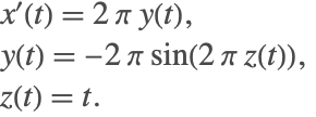
In general, a system of ordinary differential equations (ODEs) can be expressed in the normal form,
The derivatives of the dependent variables ![]() are expressed explicitly in terms of the independent transient variable
are expressed explicitly in terms of the independent transient variable ![]() and the dependent variables
and the dependent variables ![]() . As long as the function
. As long as the function ![]() has sufficient continuity, a unique solution can always be found for an initial value problem where the values of the dependent variables are given at a specific value of the independent variable.
has sufficient continuity, a unique solution can always be found for an initial value problem where the values of the dependent variables are given at a specific value of the independent variable.
With differential-algebraic equations (DAEs), the derivatives are not, in general, expressed explicitly. In fact, derivatives of some of the dependent variables typically do not appear in the equations. For example, the following equation
does not explicitly contain any derivatives of ![]() . Such variables are often referred to as algebraic variables.
. Such variables are often referred to as algebraic variables.
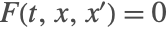
The general form of a system of DAEs is
Solving systems of DAEs often involves many steps. The flow chart shown below indicates the general process associated with solving DAEs in NDSolve.

Flow chart of steps involved in solving DAE systems in NDSolve.
Generally, a system of DAEs can be converted to a system of ODEs by differentiating it with respect to the independent variable ![]() . The index of a DAE is the number of times needed to differentiate the DAEs to get a system of ODEs.
. The index of a DAE is the number of times needed to differentiate the DAEs to get a system of ODEs.
The DAE solver methods built into NDSolve work with index-1 systems, so for higher-index systems an index reduction may be necessary to get a solution. NDSolve can be instructed to perform that index reduction. When a system is found to have an index greater than 1, NDSolve generates a message and number of steps need to be taken in order to solve the DAE.
As a first step for high-index DAEs, the index of the system needs to be reduced. The process of differentiating to reduce the index, referred to as index reduction, can be done in NDSolve with a symbolic process.
The process of index reduction leads to a new equivalent system. In one approach, this new system is restructured by substituting new (dummy) variables in place of the differentiated variables. This leads to an expanded system that then can be uniquely solved. Another approach for restructuring the system involves differentiating the original system ![]() number of times until the differentials for all the variables are accounted for. The preceding
number of times until the differentials for all the variables are accounted for. The preceding ![]() differentiated systems are treated as invariants.
differentiated systems are treated as invariants.
In order to solve the new index-reduced system, a consistent set of initial conditions must be found. A system of ODEs in normal form, ![]() , can always be initialized by giving values for
, can always be initialized by giving values for ![]() at the starting time. However, for DAEs it may be difficult to find initial conditions that satisfy the residual equation
at the starting time. However, for DAEs it may be difficult to find initial conditions that satisfy the residual equation ![]() ; this amounts to solving a nonlinear algebraic system where only some variables may be independently specified. This will be discussed in further detail in a a later section. Furthermore, the initialization needs to be consistent. This means that the derivatives of the residual equations
; this amounts to solving a nonlinear algebraic system where only some variables may be independently specified. This will be discussed in further detail in a a later section. Furthermore, the initialization needs to be consistent. This means that the derivatives of the residual equations ![]() also need to be satisfied. Commonly, higher-index systems are harder to initialize. In this case NDSolve cannot, in general, see how the components of
also need to be satisfied. Commonly, higher-index systems are harder to initialize. In this case NDSolve cannot, in general, see how the components of ![]() interact and is thus not able do an automatic index reduction. NDSolve, however, has a number of different methods, accessible via options, to perform index reduction and find a consistent initialization of DAEs.
interact and is thus not able do an automatic index reduction. NDSolve, however, has a number of different methods, accessible via options, to perform index reduction and find a consistent initialization of DAEs.
The remainder of this document is structured in the following manner: first, some terminology around indices of DAEs is introduced. Following that, the next section treats solving of index-1 DAEs. Next, methods for index reduction of higher-order index DAEs are presented. Consistent initialization of DAEs is treated subsequently. In addition to the examples in the sections mentioned so far, an entire last section with additional examples is given.
Index of a DAE
For a general DAE system ![]() , the index of the system refers to the minimum number of differentiations of part or all the equations in the system that would be required to solve for
, the index of the system refers to the minimum number of differentiations of part or all the equations in the system that would be required to solve for ![]() uniquely in terms of
uniquely in terms of ![]() and
and ![]() . Note that there are many slightly different concepts of index in the literature; for the purpose of this document the preceding concept will be used.
. Note that there are many slightly different concepts of index in the literature; for the purpose of this document the preceding concept will be used.
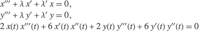
In order to get a differential equation for ![]() , the first equation must be differentiated once. This leads to the new system
, the first equation must be differentiated once. This leads to the new system
The differentiated system now contains ![]() , which must be accounted for. To get an equation for
, which must be accounted for. To get an equation for ![]() , the second equation must now be differentiated three times. This leads to
, the second equation must now be differentiated three times. This leads to
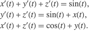
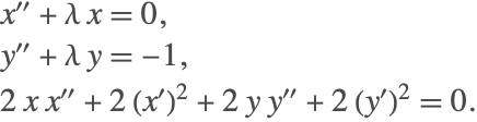
Since part of the system had to be differentiated three times to get a derivative equation for ![]() , the index of the DAE is 3. The final differentiated system is said to be an index-0 system. To see ODEs that are obtained by the differentiations, you can perform appropriate substitutions, in this case subtracting the second equation from the first. The resulting equation can be written as
, the index of the DAE is 3. The final differentiated system is said to be an index-0 system. To see ODEs that are obtained by the differentiations, you can perform appropriate substitutions, in this case subtracting the second equation from the first. The resulting equation can be written as
Similarly, the index-1 system can be found by differentiating the second equation twice, resulting in the following system
It is typical to reduce the index of the system to 1, since the underlying integration routines can handle them efficiently.
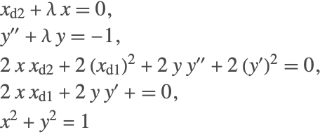
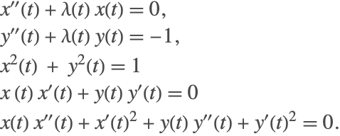
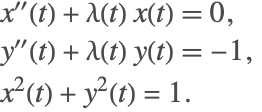
The index of a DAE may not always be obvious. Consider a system that may exhibit index-1 or index-2 behavior, depending on what the initial conditions are.
For this DAE, the initial conditions are not free; the second equation requires that ![]() be either 0 or 1.
be either 0 or 1.
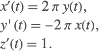
If ![]() , then the two remaining equations make an index-1 system, since differentiation of the third equation gives a system of two ODEs
, then the two remaining equations make an index-1 system, since differentiation of the third equation gives a system of two ODEs
While the initial condition for ![]() , the initial condition for
, the initial condition for ![]() can be varied.
can be varied.
On the other hand, if ![]() , then the two remaining equations make an index-2 system. Differentiating the third equation gives
, then the two remaining equations make an index-2 system. Differentiating the third equation gives ![]() , and substituting into the first equation gives
, and substituting into the first equation gives ![]() , which needs to be differentiated to get an ODE
, which needs to be differentiated to get an ODE
There are also no additional degrees of freedom in the initial conditions, since ![]() and
and ![]() .
.
Both the number of initial conditions needed and the index of a DAE may influence the actual solution being found.
Treatment of Differential Equations
In order to solve a differential equation, NDSolve converts the user-specified system into one of three forms. This step is quite important because depending on how the system is constructed, different integration methods are chosen.
You may specify in which form to represent the equations by using the option Method->{"EquationSimplification"->simplification}. The following simplification methods can be specified for the "EquationSimplification" option.
| Automatic | try to solve the system symbolically in the form |
| "Solve" | solve the system symbolically in the form |
| "MassMatrix" | reduce the system to the form |
| "Residual" | subtract right-hand sides of equations from left-hand sides to form a residual function |
Equation simplification methods.
By default, an attempt is made to solve for the derivatives ![]() explicitly in terms of the independent and dependent variables
explicitly in terms of the independent and dependent variables ![]() and
and ![]() . For efficiency purposes, NDSolve first attempts to try to find the explicit system by using LinearSolve. If that fails, however, then the system is solved symbolically using Solve.
. For efficiency purposes, NDSolve first attempts to try to find the explicit system by using LinearSolve. If that fails, however, then the system is solved symbolically using Solve.
Using the "Solve" method is the same as the default when a symbolic solution is found.
When the system is put in a residual form, the derivatives are represented by a new set of variables that are generated to be unique symbols. You can get the correspondence between these working variables and the specified variables using the "Variables" and "WorkingVariables" properties of NDSolveStateData.
The process of generating an explicit system of ODEs may sometimes become expensive due to the symbolic treatment of the system. For this reason, there is a time constraint of one second put on obtaining the equations. If that time is exceeded, then NDSolve generates a message and attempts to solve the system as a DAE.
The following method options can be specified to the simplification methods to better control the behavior of "EquationSimplification".
option name | default value | |
| "TimeConstraint" | 1 | maximum time in seconds allowed for Solve to explicitly solve for the derivatives |
| "SimplifySystem" | False | whether to simplify by obtaining analytic solutions for as many dependent variables as possible |
As indicated by the message, NDSolve did not solve explicitly for the derivatives because Solve had exceeded the default time constraint of one second. The amount of time that NDSolve spends on obtaining an explicit expression can be controlled using the option "TimeConstraint".
In the preceding example, due to the square terms in the first equation, four possible solutions are encountered. When solving as a DAE, the numerical solution will only follow one of these solution branches, depending on how it is initialized.
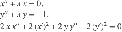
To demonstrate the usage of the method option "SimplifySystem", consider the following example:
An analytic solution for the above system can be obtained by substituting ![]() into the first equation to get a solution for
into the first equation to get a solution for ![]() , which in turn is substituted into the second equation to give a solution for
, which in turn is substituted into the second equation to give a solution for ![]() . The final solution for the system is
. The final solution for the system is
NDSolve cannot solve this system without first performing index reduction of the system and forming a new equivalent system of ODEs. This could prove to be expensive. When the suboption "SimplifySystem" is turned on, NDSolve detects any variable for which an analytic expression/solution can be found and performs repeated substitutions back into the original system. This results in the original system being either simplified or in some cases (like the above) getting back analytic solutions.
If an analytic solution does not exist for certain variables, then NDSolve will return an interpolating function as the solution.
With the suboption turned on, constant parameters can also be directly substituted into the system.
DAE Solution Methods
There are a variety of solution methods built into NDSolve for solving DAEs.
Two methods work with the general residual form of index-1 DAEs, ![]() .
.
- IDA—(Implicit Differential-Algebraic solver from the SUNDIALS package) based on backward differentiation formulas (BDF)
- StateSpace—implicitly solves
 for derivatives
  to use an underlying ODE solver
If the system has index higher than 1, both of these solvers typically fail. To accurately solve such systems, index reduction is needed. Note that index-1 systems can be reduced to ODEs, but it is often more efficient to use one of the solvers above.
NDSolve also has some solvers that work with DAEs that can be reduced to special forms.
- Projection—for ODEs
 with invariants
The following subsections describe some aspects of using these methods for DAEs.
ODEs with Invariants
It is common to encounter DAEs of the form
where ![]() is an invariant that is consistent with the differential equations.
is an invariant that is consistent with the differential equations.
When a system of DAEs is converted to ODEs via index reduction, the equations that were differentiated to get the ODE form are consistent with the ODEs, and it is typically important to make sure those equations are well satisfied as the solution is integrated.
Such systems have more equations than unknowns and are overdetermined unless the constraints are consistent with the ODEs. NDSolve does not handle such DAEs directly because it expects a system with the same number of equations and dependent variables. In order to solve such systems, the "Projection" method built into NDSolve handles the invariants by projecting the computed solution onto ![]() after each time step. This ensures that the algebraic equations are satisfied as the solution evolves.
after each time step. This ensures that the algebraic equations are satisfied as the solution evolves.
An example of such a constrained system is a nonlinear oscillator modeling the motion of a pendulum.
Note that the differential equation is effectively the derivative of the invariant, so one way to solve the equation is to use the invariant.
Solving Systems with a Mass Matrix
When the derivatives appear linearly, a differential system can be written in a form
where ![]() is a matrix often referred to as a mass matrix. Sometimes
is a matrix often referred to as a mass matrix. Sometimes ![]() is also referred to as a damping matrix. If the matrix is nonsingular, then it can be inverted and the system can be solved as an ODE. However, in the presence of a singular matrix, the system can be solved as a DAE. In either case, it may be advantageous to take advantage of the special form.
is also referred to as a damping matrix. If the matrix is nonsingular, then it can be inverted and the system can be solved as an ODE. However, in the presence of a singular matrix, the system can be solved as a DAE. In either case, it may be advantageous to take advantage of the special form.
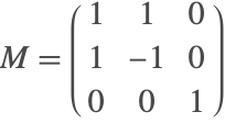
The system describing the motion of a particle on a cylinder
can be expressed in mass matrix form with
Index Reduction for DAEs
The built-in solvers for DAEs in NDSolve currently handle index-1 systems of DAEs fully automatically. For higher-index systems, an index reduction is necessary to get to a solution. This index reduction can be performed by giving appropriate options to NDSolve.
NDSolve uses symbolic techniques to do index reduction. This means that if your DAE system is expressed in the form ![]() , where NDSolve cannot see how the components of
, where NDSolve cannot see how the components of ![]() interact and compute symbolic derivatives, the index reduction cannot be done, and for this reason NDSolve does not do index reduction, by default.
interact and compute symbolic derivatives, the index reduction cannot be done, and for this reason NDSolve does not do index reduction, by default.
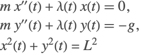
For an example, consider the classic DAE describing the motion of a pendulum:
where there is a mass ![]() at the point
at the point ![]() constrained by a string of length
constrained by a string of length ![]() .
. ![]() is a Lagrange multiplier that is effectively the tension in the string. For simplicity in the description of index reduction, take
is a Lagrange multiplier that is effectively the tension in the string. For simplicity in the description of index reduction, take ![]() . The figure shows the schematic of the pendulum system.
. The figure shows the schematic of the pendulum system.

Sketch of the forces acting on a pendulum.
If the index of the system is not obvious from the equations, one thing to do is try it in NDSolve, and if the solver is not able to solve it, in many cases it is able to generate a message indicating what the index appears to be for the initial conditions specified.
The message indicates that the index is 3, indicating that index reduction is necessary to solve the system. Note that a complete consistent initialization is used here to avoid possible issues with initialization. This aspect of the solution procedure is treated in "Consistent Initialization of DAEs" with more detail.
The option setting Method->{"IndexReduction"->{irmeth,iropts}} is used to specify that NDSolve uses index reduction method irmeth with general index reduction options iropts.
| None | no index reduction (default) |
| Automatic | choose the method automatically |
| "Pantelides" | graph-based Pantelides algorithm |
| "StructuralMatrix" | structural matrix-based algorithm |
The following options can be given for all index reduction methods.
| "ConstraintMethod" | Automatic | how to handle constraints from specified system |
| "IndexGoal" | Automatic | index to reduce to (1 or 0) |
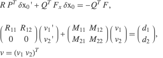
Index reduction is done by differentiating equations in the DAE system. Suppose that an equation eqn is differentiated during the process of index reduction so that deqn=![]() eqn is included in the system in place of eqn. Once the differentiation has been done, the differentiated equations comprise a fully determined system and can be solved on their own. However, it is typically important to incorporate the original equations in the system as constraints. How this is done is controlled by the "ConstraintMethod" index reduction option.
eqn is included in the system in place of eqn. Once the differentiation has been done, the differentiated equations comprise a fully determined system and can be solved on their own. However, it is typically important to incorporate the original equations in the system as constraints. How this is done is controlled by the "ConstraintMethod" index reduction option.
| None | do not keep the original equations as constraints and just solve with the differentiation equations |
| "DummyDerivatives" | use the method of Mattson and Soderlind [MS93] to replace some derivatives with algebraic variables (dummy derivatives) |
| "Projection" | reduce the index to 0 to get an ODE and use the "Projection" time integration method with the original equations that were differentiated as invariants |
In the numerical solution with just the differentiated equations, the length of the pendulum is drifting away from 1. Incorporating the original equations into the solution as constraints is an important aspect of index reduction.
The next two sections will describe index reduction algorithms, followed by an explanation of constraint methods that can be used in NDSolve.
Index Reduction Algorithms
NDSolve has two algorithms for doing index reduction, the Pantelides and the structural matrix methods. Both of these methods use the symbolic form of the equations to determine which equations to differentiate and then use symbolic differentiation to get the differentiated system.
Both methods make use of the concept of structural incidence in the equations; in particular, if variable ![]() appears explicitly in equation
appears explicitly in equation ![]() , then
, then ![]() is termed incident in
is termed incident in ![]() . The structural incidence matrix is the matrix with elements
. The structural incidence matrix is the matrix with elements ![]() if
if ![]() is incident in
is incident in ![]() and otherwise
and otherwise ![]() . A DAE system has structural index 1 if the structural incidence matrix can be reordered so that there are 1s along the diagonal. The existence of such a reordering means that there is a matching between equations and variables such that there is one equation for every variable.
. A DAE system has structural index 1 if the structural incidence matrix can be reordered so that there are 1s along the diagonal. The existence of such a reordering means that there is a matching between equations and variables such that there is one equation for every variable.
The Pantelides algorithm works with a graph based on the incidence that can be very efficient even for extremely large systems.
Note that the structural index may be smaller than the actual index of the system. In the real system, terms that are structurally present may vanish along some solutions or the Jacobian matrix may be singular. The structural matrix method tries to take into account the possibility of singularities in the Jacobian and will do a better job of index reduction for some systems, but at the cost of greater computational expense.
The next section introduces a command for getting the structural incidence matrix that is useful for the descriptions of the Pantelides and structural matrix algorithms that follow in the subsequent sections.
Structural Incidence
| NDSolve`StructuralIncidenceArray[eqns,vars] | return a SparseArray that has the pattern of the structural incidence matrix for the variables vars in the equations eqns |
Getting the structural incidence.
Note that the SparseArray contains just the nonzero pattern that uses less memory and indicates it represents the pattern of incidence. It can be converted to a SparseArray with 1s using ArrayRules.
The system has structural index 1, since no reordering is needed to avoid zeros along the diagonal.
If the structural incidence with respect to the derivative variables can be arranged to avoid zeros on the diagonal, then the system is index 0.
There is no reordering that will avoid zeros on the diagonal. However, if the second equation is differentiated it is possible.
The differentiated system has structural index 0, verifying that the original system was index 1.
Consider the constrained pendulum (2) as another example.
The matrix cannot be reordered to avoid zeros on the diagonal, so the index is greater than 1.
Note that the function NDSolve`StructuralIncidenceArray just does a literal matching on the FullForm of the expression to check for the incidence. It does not do any checking to see if your equations or variables are properly formed.
This is a full matrix because the FullForm of x'[t] is Derivative[1][x][t] that contains x.
Pantelides Method
The method proposed by Pantelides [P88] is a graph theoretical method that was originally proposed for finding consistent initialization of DAEs. It works with a bipartite graph of dependent variables and equations, and when the algorithm can find a traversal of the graph, then the system has been reduced to index at most 1. A traversal in this sense effectively means an ordering of variables and equations so that the graph's incidence matrix has no zeros on the diagonal.
When the bipartite graph does not have a complete traversal, the algorithm effectively augments the path by differentiating equations, introducing new variables (derivatives of previous variables) in the process. Unless the original system is structurally singular, the algorithm will terminate with a traversal. Generally, the algorithm does only the differentiations needed to get the traversal, but since it is a greedy algorithm, it is not always the minimal number.
It is beyond the scope of this documentation to describe the algorithm in detail. The implementation built into the Wolfram Language follows the algorithm outlined in [P88] fairly closely. It uses Graph to efficiently implement the graph computations and symbolically differentiates the equations with D when differentiation is called for.
When there is a traversal of the system, it is then possible to find an ordering for the variables and equations such that the incidence matrix is in block lower triangular (BLT) form. The BLT form is used in setting up the dummy derivative method for maintaining constraints and also in the "StateSpace" time integration method. A description of the BLT ordering is included in "State Space Method for DAEs".
To begin index reduction on the constrained pendulum system (2), consider the variables ![]() . Generally, start with the highest-order derivative that appears in the equations. As a reminder, the pendulum equations are
. Generally, start with the highest-order derivative that appears in the equations. As a reminder, the pendulum equations are
and the graph incidence matrix with respect to the highest-order derivative is
The incidence matrix is constructed by checking the presence of a variable in an equation. If the variable exists in the equation, a weight of 1 is given; if not then 0 is specified. So checking for the variables ![]() in the first equation gives
in the first equation gives ![]() (as seen in the first row of the incidence matrix).
(as seen in the first row of the incidence matrix).
From the first incidence matrix, it is found that there is no traversal. The last equation is differentiated twice
This can be reordered so that there is no zero on the diagonal by swapping the first and last equations, resulting in the incidence matrix
The resulting system has index 1 since ![]() still appears as an algebraic variable and does not contain a derivative in the differentiated system. Differentiating the system one more time will provide a differential system for
still appears as an algebraic variable and does not contain a derivative in the differentiated system. Differentiating the system one more time will provide a differential system for ![]() . Therefore, the index of the original system is indeed 3.
. Therefore, the index of the original system is indeed 3.
As a first approach, the system with the twice-differentiated equation can be solved directly.
The original pendulum length constraint is not being satisfied well; in fact, it stretches! The constraints are not satisfied well because the new system does not identically represent the original system. This can be seen by the fact that the new system does not contain the original constraint of ![]() , but rather its differentiated equations.
, but rather its differentiated equations.
To model the original dynamics of the system with the new system, additional equations must be satisfied. However, including additional equations leads to more equations than unknowns. To address this issue, the method of dummy derivatives is used, so that the index-reduced system becomes balanced.
The Pantelides algorithm is efficient because it can use graph algorithms with well-controlled complexity even for very large problems. However, since it is based solely on incidence, there can be issues with systems that lead to Jacobians that are singular. The structural matrix method may be able to resolve such cases, but may have larger computational complexity for large systems.
Structural Matrix Method
The structural matrix algorithm is an alternative to the Pantelides algorithm. The structural matrix method follows from the work of Unger [UKM95] and Chowdhary et al. [CKL04]. The graph-based algorithms such as the Pantelides algorithm rely on traversals to perform index reduction. However, they do not account for the fact that sometimes there may be variable cancellations in a particular system. This leads to the algorithm underestimating the index of the system. If a DAE has not been correctly reduced to an index-0 or index-1 system, then the numerical integration may fail or may produce an incorrect result.
As an example of variable cancellation that is not taken into account by Pantelides's method, consider the following DAE
To perform index reduction, as a first step the second equation is differentiated once, giving
The Pantelides algorithm stops after the first differentiation because it finds derivatives for the variables ![]() and finds a traversal. Since all the derivatives are found from the first differentiation, the Pantelides algorithm estimates the index of the system to be 0. An index-0 system is equivalent to a system of ODEs. The Jacobian of the derivatives for the differentiated system is found to be
and finds a traversal. Since all the derivatives are found from the first differentiation, the Pantelides algorithm estimates the index of the system to be 0. An index-0 system is equivalent to a system of ODEs. The Jacobian of the derivatives for the differentiated system is found to be
and is clearly singular. By simple substitutions, it is possible to see that the differentiated system is equivalent to
This implies that in order to get a system of ODEs, a second differentiation must be done for the second equation. This results in the final system
The above system has a nonsingular Jacobian for the derivatives. The above system is now correctly index 0 and a system of ODEs can be formed from it. Since two differentiations were required, the actual index of the system is 2 (instead of 1).
Unlike the Pantelides algorithm, the structural matrix method accounts for all cancellations associated with the linear terms. The steps of the method are demonstrated using the pendulum example (2) described as a first-order system
As a first step, two matrices ![]() and
and ![]() are constructed. The matrices are incidence matrices associated with the derivatives
are constructed. The matrices are incidence matrices associated with the derivatives ![]() and the variables
and the variables ![]() , respectively. For the above system, the matrix
, respectively. For the above system, the matrix ![]() is given as
is given as
The matrix above contains a ![]() as some of its entries. The
as some of its entries. The ![]() is used as a placeholder, indicating that the variables in that equation (row) are present in the equation in a nonlinear fashion. Notice that for the second equation, the terms
is used as a placeholder, indicating that the variables in that equation (row) are present in the equation in a nonlinear fashion. Notice that for the second equation, the terms ![]() and
and ![]() appear as products. Therefore, the first and last columns in the second row are marked with a
appear as products. Therefore, the first and last columns in the second row are marked with a ![]() .
.
Once the matrices are constructed, the objective is to try and convert the system of DAEs into a system of ODEs. In order to do that, the rank of the matrix ![]() must be full. To achieve this, equations that need to be differentiated are first identified. In this case, it is the last equation. After differentiation, the structural matrices are
must be full. To achieve this, equations that need to be differentiated are first identified. In this case, it is the last equation. After differentiation, the structural matrices are
The last column of the matrix ![]() has changed due to the differentiations. To see this more clearly, consider the last equation in (3). Differentiating the equation gives
has changed due to the differentiations. To see this more clearly, consider the last equation in (3). Differentiating the equation gives ![]() . Notice now that the terms
. Notice now that the terms ![]() are present in the equation and appear in a nonlinear manner. Therefore the incidence row associated with the derivatives is
are present in the equation and appear in a nonlinear manner. Therefore the incidence row associated with the derivatives is ![]() , and the incidence row associated with the variables is
, and the incidence row associated with the variables is ![]() .
.
The next step involves matrix factorization in the form of Gaussian elimination for the matrix ![]() . The elements in the last row of
. The elements in the last row of ![]() can be eliminated by making use of rows 1 and 3. This elimination also affects the rows of the matrix
can be eliminated by making use of rows 1 and 3. This elimination also affects the rows of the matrix ![]() . Multiplying the first row of
. Multiplying the first row of ![]() with
with ![]() and subtracting it from the last row leads to
and subtracting it from the last row leads to
Multiplying the third row with ![]() and subtracting it from the last row gives
and subtracting it from the last row gives
The matrix ![]() is still rank deficient and therefore the above steps must be repeated. A second iteration leads to the system
is still rank deficient and therefore the above steps must be repeated. A second iteration leads to the system
A third iteration leads to the system
The matrix ![]() is now a full-rank matrix. Therefore the iterations are stopped. Since three iterations were needed to get a full-rank matrix for
is now a full-rank matrix. Therefore the iterations are stopped. Since three iterations were needed to get a full-rank matrix for ![]() , the index of the system is 3. Note that unlike the Pantelides method, the structural matrix algorithm explicitly operates on the incidence matrices.
, the index of the system is 3. Note that unlike the Pantelides method, the structural matrix algorithm explicitly operates on the incidence matrices.
The next examples demonstrate the advantage and differences of the structured matrix method over the Pantelides algorithm. Consider the linear system
This fails because there is a singular Jacobian matrix. Very commonly the messages NDSolve::nderr or NDSolve::ndcf are issued by the solver when the DAE's index is greater than 1.
The exact solutions are ![]() and
and ![]() . Comparing the exact and numerical results, it is found that the computed solution is quite accurate.
. Comparing the exact and numerical results, it is found that the computed solution is quite accurate.
Next, consider the effect of under- or overestimating the index of a system. Consider the linear system
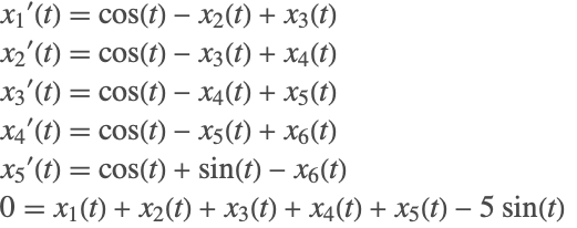
The exact solution for all the variables is ![]() . This is an index-4 system. The Pantelides algorithm estimates the index to be 2.
. This is an index-4 system. The Pantelides algorithm estimates the index to be 2.
The solver encounters a convergence failure because the Jacobian is singular.
There are certain tests that NDSolve performs to determine which index reduction method to use. For this case, using the option Automatic, NDSolve picks the structural matrix algorithm.
If the system is forced to be treated as index 0, integration can be performed. However, in the absence of incorrect estimation of the index, the results can be wildly off because the solution is being computed for a completely different manifold.
Since the exact solution is known for this problem, it is desirable to see the difference between the numerical solution and the exact result.
Due to the underestimation of the index of the system, the necessary differentiations are not carried out, leading to the solution's being approximated on an incorrect manifold. The structural matrix method, on the other hand, is able to correctly identify the index of the system.
The structural matrix method does handle such systems much better. It is, however, important to note that there is a price to be paid for the rigor of accounting for cancellations. The structural matrix method relies on generating, maintaining, and operating on matrices, which has a significant computational overhead compared to the Pantelides algorithm. The algorithm is therefore only suited for small-to-medium-scale problems.
Constraint Methods
Dummy Derivatives
The purpose of the dummy derivative method is to introduce algebraic variables so that the combined system of original equations and equations that have been differentiated for index reduction is not overdetermined.
Consider the pendulum system (2) again.
Note that for this example the "ConstraintMethod"->"DummyDerivatives" was included for emphasis and is not needed, since trying to use dummy derivatives is the default.
Now the constraints are very well satisfied.
The main idea behind the dummy derivative method of Mattson and Söderlind [MS93] is to introduce new variables that represent derivatives, thus making it possible to reintroduce constraint equations without getting an overdetermined system.
Recall the index-reduced equations for the system (2) were
with the two constraints from the third equation and its first derivative
Let ![]() and
and ![]() be algebraic variables that replace
be algebraic variables that replace ![]() and
and ![]() , respectively. Then, with the constraints included, the entire system in these variables is given by
, respectively. Then, with the constraints included, the entire system in these variables is given by
and the incidence matrix with variables ![]() is
is
that can be reordered to have a nonzero diagonal.
In general, the algorithm can be applied to any index-reduced DAE; however, while integrating the system, the solver may encounter singularities.
The above system cannot complete integration because the system becomes singular when ![]() .
.
From the plot it can be seen that NDSolve is getting stuck when ![]() is becoming 0. When
is becoming 0. When ![]() is 0, several terms drop out, the incidence matrix becomes singular, and a nonzero diagonal can no longer be found, so the dummy derivative system effectively has index
is 0, several terms drop out, the incidence matrix becomes singular, and a nonzero diagonal can no longer be found, so the dummy derivative system effectively has index ![]() along solutions that go through
along solutions that go through ![]() .
.
Consider an alternative dummy derivative replacement, i.e. ![]() and
and ![]() to replace
to replace ![]() and
and ![]() . Unfortunately, the system with this replacement becomes singular at
. Unfortunately, the system with this replacement becomes singular at ![]() .
.
The remedy is to use dynamic state selection such that ![]() and
and ![]() replace
replace ![]() and
and ![]() when
when ![]() is away from 0 and switch dynamically to the system using
is away from 0 and switch dynamically to the system using ![]() and
and ![]() to replace
to replace ![]() and
and ![]() when
when ![]() becomes too small. NDSolve automatically uses WhenEvent with state replacement rules to handle dynamic state selection with dummy derivatives if necessary. The exact details of the dynamic state selection are beyond the scope of this tutorial. A detailed explanation can be found in Mattson and Söderlind [MS93].
becomes too small. NDSolve automatically uses WhenEvent with state replacement rules to handle dynamic state selection with dummy derivatives if necessary. The exact details of the dynamic state selection are beyond the scope of this tutorial. A detailed explanation can be found in Mattson and Söderlind [MS93].
Projection
The alternative to using dummy derivatives is to reduce the index to 0 so there is a system of ODEs and use projection to ensure that the original constraints are satisfied.
For the pendulum system (2), the index of the system is 3. This means that in order to get an ordinary differential equation for all the variables, the first and second equations must be differentiated once, while the third equation must be differentiated three times. This results in
that can be solved for the derivatives ![]() ,
, ![]() , and
, and ![]() . (NDSolve will also reduce the system to first order automatically.)
. (NDSolve will also reduce the system to first order automatically.)
In order to correctly represent the dynamics of the system, the first ![]() differentiated equation must also be taken into account. These equations are
differentiated equation must also be taken into account. These equations are
The above equations are treated as invariant equations that must be satisfied at each time step. Since the ODE system was derived from differentiating these equations, the constraints are guaranteed to be consistent with the ODEs, so the system can be solved using the "Projection" time integration method with the constraints as invariants.
This can be done automatically using the built-in index reduction method in NDSolve directly.
With this method, the original constraints are typically satisfied up to the local tolerances for NDSolve specified by the PrecisionGoal and AccuracyGoal options.
The system has additional invariants that should also be satisfied. One of these is the conservation of energy that can be expressed by ![]() . Because the projection method only projects at the ends of the time steps, this is the most appropriate place to do the comparison.
. Because the projection method only projects at the ends of the time steps, this is the most appropriate place to do the comparison.
Index Reduction of Partial Differential Algebraic Equations (PDAE):
Consider the following system of partial differential equations:
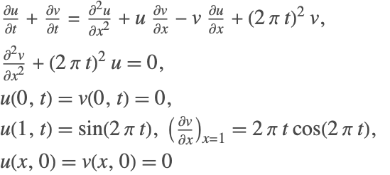
In the above system, the second PDE does not contain a time derivative component for any of the variables. Therefore, NDSolve cannot solve this system using method of lines because the resulting mass-matrix will be singular and the system has an index of 1. To reduce the index of the system, the above system is represented in a matrix-vector form as
The terms ![]() represent the matrices obtained by discretizing the spatial derivatives and the terms
represent the matrices obtained by discretizing the spatial derivatives and the terms ![]() represent the vectors obtained by discretizing the variables
represent the vectors obtained by discretizing the variables ![]() at discrete spatial intervals
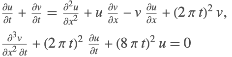
at discrete spatial intervals ![]() . Index reduction is performed on the new system using the index-reduction methods described above. The resulting index-reduced system is
. Index reduction is performed on the new system using the index-reduction methods described above. The resulting index-reduced system is
The spatial derivatives are now reintroduced back into the system to give
The resulting system can then be solved using traditional methods available in NDSolve.
Note that 200 points were used for the spatial discretization because the default spatial grid spacing based on the constant initial condition is insufficient to handle the variation the solution develops over time.
It is important to note that the index reduction is performed in the time derivative, so no new boundary conditions are needed or added to the system. However, if the PDAE is found to be of high index, then additional initial conditions may be needed.
Consistent Initialization of DAEs
A system of differential algebraic equations (DAEs) can be represented in the most general form as
which may include differential equations and algebraic constraints. In order to obtain a solution for ![]() , a set of consistent initial conditions for
, a set of consistent initial conditions for ![]() and
and ![]() is needed to start the integration. A necessary condition for consistency is that the initial conditions satisfy
is needed to start the integration. A necessary condition for consistency is that the initial conditions satisfy ![]() However, this condition alone may not be sufficient, since differentiating the original equations produces new equations that also need to be satisfied by the initial conditions. The task therefore is to try and find initial conditions that satisfy all necessary consistency conditions. The problem of finding consistent initial conditions can be one of the most difficult parts of solving a DAE system.
However, this condition alone may not be sufficient, since differentiating the original equations produces new equations that also need to be satisfied by the initial conditions. The task therefore is to try and find initial conditions that satisfy all necessary consistency conditions. The problem of finding consistent initial conditions can be one of the most difficult parts of solving a DAE system.
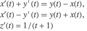
Consider the following linear DAE problem:
The DAE has derivatives for ![]() . This would suggest that in order to uniquely solve this problem, initial conditions for
. This would suggest that in order to uniquely solve this problem, initial conditions for ![]() need to be specified. However, you cannot specify any arbitrary initial conditions to the variables, since there is a unique set of consistent initial conditions. Differentiating the algebraic equation once leads to
need to be specified. However, you cannot specify any arbitrary initial conditions to the variables, since there is a unique set of consistent initial conditions. Differentiating the algebraic equation once leads to ![]() Substituting in the second equation gives the solution for
Substituting in the second equation gives the solution for ![]() . Differentiating
. Differentiating ![]() and substituting into the first equation gives the solution for
and substituting into the first equation gives the solution for ![]() This shows that the solution for the DAE system is fixed, and therefore the initial conditions are also fixed, and the only consistent set of initial conditions for
This shows that the solution for the DAE system is fixed, and therefore the initial conditions are also fixed, and the only consistent set of initial conditions for ![]() is
is ![]() It is important to note that the constraints on the initial conditions are not obvious, in general making the problem of finding consistent initial conditions quite challenging.
It is important to note that the constraints on the initial conditions are not obvious, in general making the problem of finding consistent initial conditions quite challenging.
In some cases, you may just want to get a consistent initialization for a DAE problem and not compute the solution further. This can be done with NDSolve by specifying the endpoint of the time integration to be the same as the time where the initial condition is specified. Such a step is generally helpful when you need to examine just the starting conditions without having to perform the complete integration.
NDSolve provides several methods for DAE initialization. The method m can be specified using Method->{"DAEInitialization"->m}.
| Automatic | determine the method to use automatically |
| "Collocation" | use a collocation method; this algorithm can be used for initialization of high-index systems |
| "QR" | use a QR decomposition-based algorithm for index-1 systems |
| "BLT" | use a Block Lower Triangular ordering (BLT) approach for index-1 systems |
Methods for DAE initialization.
The collocation method is designed to handle the DAE system as a residual black box and tries to achieve the objective of satisfying the residual over a small interval near the point of initialization. This feature allows the method to be used to handle initialization of high-index systems. However, since the algorithm does not analyze the DAE system, the structure of the system cannot be exploited for computational efficiency. This makes the algorithm slower than the other methods.
The QR and BLT methods are designed specifically to be used for index-1 and index-0 systems. The QR method relies on decomposing the Jacobian of the derivative to generate two decoupled subsystems such that the initial conditions for the variables and their derivatives are computed iteratively. This makes the method quite efficient and robust.
The BLT method relies on examining the structure of the DAE system and splits the original system into a number of smaller subsystems such that each of these subsystems can be solved efficiently. This method results in dealing with much smaller Jacobian matrices (compared to the entire system) and thus is computationally efficient for large systems.
The following sections give details about how NDSolve obtains consistent initial conditions for DAEs using different algorithms.
Collocation Method
The basic collocation algorithm makes use of expanding the dependent variables ![]() in terms of basis functions
in terms of basis functions ![]() as
as
In order to obtain ![]() and
and ![]() , one tries to enforce the condition that
, one tries to enforce the condition that ![]() is satisfied at
is satisfied at ![]() collocation points,
collocation points, ![]() , in time. To achieve this, the implicit DAE is linearized as
, in time. To achieve this, the implicit DAE is linearized as
where ![]() and
and ![]() denote the Jacobian of
denote the Jacobian of ![]() with respect to
with respect to ![]() and
and ![]() , respectively:
, respectively:
Applying this linearization to ![]() collocation points in time, a system of linear equations is obtained for the coefficients
collocation points in time, a system of linear equations is obtained for the coefficients ![]() , which is solved iteratively using Newton's method.
, which is solved iteratively using Newton's method.
where ![]() is obtained using a line search method. If there are
is obtained using a line search method. If there are ![]() coefficients and
coefficients and ![]() collocation points, then you are dealing with an
collocation points, then you are dealing with an ![]() ×
×![]() system of linear equations in (5).
system of linear equations in (5).
For high-index systems that have not been index reduced, NDSolve automatically tries to initialize the system using the collocation algorithm. Consider the pendulum system (2)
In order to start integration of the system, the initial conditions for ![]() must be known. For such systems,
must be known. For such systems, ![]() would represent some physical property and could be assigned reasonable values. However, the value of
would represent some physical property and could be assigned reasonable values. However, the value of ![]() might not be easy to find. NDSolve can be used here to determine the appropriate values.
might not be easy to find. NDSolve can be used here to determine the appropriate values.
Notice that only partial initial conditions were given and the algorithm correctly computes all the required initial conditions.
The default settings for the collocation method have been chosen to handle initialization for a wide variety of systems; however, in some cases it is necessary to change the settings to find a consistent Initialization. The following options may be used to tune the algorithm.
collocation method option name | default value | |
| "CollocationDirection" | Automatic | chooses the direction in which the collocation points are placed; possible options include "Forward", "Backward", "Centered", "Automatic" |
| "CollocationPoints" | Automatic | number of collocation points to be used; using suboption "ExtraCollocationPoints", more grid points are added while keeping the approximation order fixed |
| "CollocationRange" | Automatic | range over which the collocation points are distributed |
| "DefaultStartingValue" | Automatic | starting value used for unspecified components in the nonlinear iterations; option can be a one-element value ig/{ig} or a list of two numbers {ig1,ig2}, where ig1,ig2 are the starting values for the variable and its derivative, respectively |
| "MaxIterations" | 100 | maximum number of iterations to be performed |
The next sections discuss these options in more detail and show in what circumstances they may help to find consistent initial conditions.
Collocation Direction
In order to perform the initialization, a set of collocation points is selected. The points can be placed on both sides, front, or back of the point of interest, using the options "Centered", "Forward", or "Backward", respectively. The following table describes the effect of choosing one of these options.
| "Forward" | collocation performed over the range |
| "Backward" | collocation performed over the range |
| "Centered" | collocation performed over the range |
"CollocationDirection" suboptions.
The term ![]() above refers to the time at which the initial condition is computed. The term
above refers to the time at which the initial condition is computed. The term ![]() is the offset value. By default, NDSolve automatically chooses the direction in which the collocation is performed.
is the offset value. By default, NDSolve automatically chooses the direction in which the collocation is performed.
The collocation direction becomes important when dealing with discontinuities.
In this case, at time ![]() ,
, ![]() is discontinuous.
is discontinuous.
NDSolve automatically sets the option for "CollocationDirection".
Applying a "CollocationDirection" of "Centered" will cause the solution to diverge.
However, using the "Forward" or "Backward" direction, you can get correct convergence by avoiding the discontinuous derivative.
In most cases, NDSolve automatically determines what the direction should be. However, if it is known that there could be discontinuities in a specific direction, then it can be avoided by using this setting. This in turn helps in reducing the computational time for NDSolve.
Collocation Points
The option "CollocationPoints" refers to the number of collocation points ![]() as indicated in (5) that will be used in the series approximation (4). Depending on the collocation points, the order
as indicated in (5) that will be used in the series approximation (4). Depending on the collocation points, the order ![]() of the series in (4) is determined. The order of the series is
of the series in (4) is determined. The order of the series is ![]() . The collocation points are essentially the Chebyshev points distributed over the collocation range.
. The collocation points are essentially the Chebyshev points distributed over the collocation range.
To illustrate the effect of "CollocationPoints", consider the following index-3 example.
The solution to the preceding DAE can be found analytically. The exact consistent initial conditions are as follows.
A manual setting of collocation points is possible. Setting "CollocationPoints"->2 is equivalent to setting ![]() in (4). This means that the solution is approximated using constant and linear basis functions.
in (4). This means that the solution is approximated using constant and linear basis functions.
Even though the iterations converged, the results are not the correct consistent initial conditions. No message is issued because they satisfy the specified equations sufficiently well.
Recall that for higher-index equations, consistent initial conditions should also work with the differentiated system.
Increasing the number of collocation points and thus allowing higher-order basis functions allows the algorithm to converge to the expected result.
Since the order of the approximation ![]() is determined by the collocation points
is determined by the collocation points ![]() , the resulting linearized system obtained in (4) will result in a square matrix, and the resulting system of linear equations can be solved efficiently using LinearSolve. However, it is quite possible that the resulting linear system may be ill conditioned or singular. Such systems are known to be sensitive and therefore can result in an unstable iteration. To resolve this issue, it is often desirable to solve an overdetermined system of equation using LeastSquares.
, the resulting linearized system obtained in (4) will result in a square matrix, and the resulting system of linear equations can be solved efficiently using LinearSolve. However, it is quite possible that the resulting linear system may be ill conditioned or singular. Such systems are known to be sensitive and therefore can result in an unstable iteration. To resolve this issue, it is often desirable to solve an overdetermined system of equation using LeastSquares.
Using the suboption "ExtraCollocationPoints", the order of the series approximation is kept equal to ![]() in (4), but the value of
in (4), but the value of ![]() in (5) is modified to
in (5) is modified to ![]() , where
, where ![]() is the extra collocation points. This, therefore, leads to an overdetermined system of equations in (5), which is solved using the least-squares method.
is the extra collocation points. This, therefore, leads to an overdetermined system of equations in (5), which is solved using the least-squares method.
Collocation Range
For very high-index systems that have not undergone index reduction, the use of a much higher collocation order might be required, along with a specification of the range in which the collocation should take place. By default, the collocation range is computed based on the working precision and the number of basis functions used in expansion.
For an example, an index-6 system for which an exact solution can be found will be used.
Typically it is necessary to use an approximation with an order higher than the index of the system. Since this is an index-6 system, you must rely on a higher-order approximation in (4). As mentioned in the previous subsection, this can be done using the option "CollocationPoints".
A solution is found, but there are significant errors from the exact consistent initial conditions. The reason for the large error is that for this example the default points are too close together and so there is noticeable numerical round-off error.
There is a close relationship between "CollocationPoints" and "CollocationRange". The collocation range is computed based on the number of collocation points so as to avoid excessive round-off errors and to accommodate higher-precision computations. Unless explicitly specified, the "CollocationRange" is computed as ![]() , where
, where ![]() is the setting of the WorkingPrecision option and
is the setting of the WorkingPrecision option and ![]() is the setting of the "CollocationPoints" method option.
is the setting of the "CollocationPoints" method option.
Specifying Initial Conditions
One of the main differences between ODEs and DAEs is that in order to integrate a system of ODEs, initial conditions for all the variables must be provided. On the other hand, for a DAE, some of these initial conditions may be fixed and must be computed directly from the system. To elaborate, consider the ODE
The initial conditions can be arbitrarily specified for the preceding system. Now consider a modification of the same system given as
This system is a DAE, but the dynamics are identical to the ODE system. The major difference now is that the initial conditions ![]() and
and ![]() are not fixed, but rather are determined by the algebraic equation.
are not fixed, but rather are determined by the algebraic equation.
The preceding example is simple enough that some determination can be made as to which variables are fixed and perhaps the initial conditions manually computed. However, as the system gets more complicated and large, you must rely on additional tools.
In certain cases, the initial conditions are completely determined by the system of equations. To illustrate this case, consider the following linear DAE system
Though the system contains two derivatives, the solution and the initial conditions are completely determined by the system. No additional information is needed.
It is important to note that it is often not possible to know which conditions are fixed and which ones are free. One approach that could be taken to gain some insight into the correct initial conditions and the order of magnitude of the initial conditions is to put the DAE equations directly into NDSolve without initial conditions and manipulate the options for the method "DAEInitialization".
Consider the pendulum system (2) represented as a first-order system. In order to uniquely define the state of the system, only two initial conditions are needed.
First, consider the case when no initial conditions are given for this DAE system. By default, the starting guess is taken to be 1 for all variables that have not been specified. Since no index reduction is performed, NDSolve automatically chooses the collocation algorithm.
It is observed that the algorithm was able to find one possible set of initial conditions out of the infinitely many possible sets. At this point, it is of course very sensitive to the starting guesses. It is also important to note that convergence of the iterations is not guaranteed.
The initial starting guess can be changed using the option "DefaultStartingValue" for the collocation method. If an initial starting guess of -1 is used, then a different set of valid solutions will be found.
As mentioned earlier, two initial conditions are sufficient to fix the state of the system. For the pendulum case, the value of ![]() and
and ![]() fixes the system.
fixes the system.
If the state is truly fixed, then the system should theoretically be insensitive to the starting initial guess.
For certain systems, the computation of initial conditions is sensitive to the starting guess. To demonstrate, consider the following system.
For this problem with x2[t]0, the general solution is {x1[t]x1[0]+t2/2,x2[t]0,x3[t]t}, so it is necessary to give x1[0] to determine the solution. By using a default value of 1 as the starting guess, the algorithm is forced to change the specified initial condition.
The code essentially switches to a different solution branch.
This happens because the default starting guess for the state ![]() is 1. During the Newton iterations, the system becomes singular because the second equation is identically satisfied, and as a result the iterations diverge. To avoid complete failure, the algorithm is forced to modify the specified condition of
is 1. During the Newton iterations, the system becomes singular because the second equation is identically satisfied, and as a result the iterations diverge. To avoid complete failure, the algorithm is forced to modify the specified condition of ![]() .
.
To avoid this behavior, a "better" starting guess can be given. Using a starting guess of -1, the iterations converge to the expected consistent initial condition.
QR Method
The QR decomposition method is based on the work of Shampine [S02]. This algorithm is intended for index-1 or index-0 systems. The algorithm makes use of the efficient QR decomposition technique to decouple the system variables and their derivatives. In doing so, at each iteration step the solution of one system is broken down into two smaller systems of equations. For an ![]() -variable DAE system, the QR algorithm needs to handle at most a matrix of size
-variable DAE system, the QR algorithm needs to handle at most a matrix of size ![]() as opposed to a matrix of size
as opposed to a matrix of size ![]() if the collocation method is used. In most cases, the algorithm only needs to handle matrices much smaller than
if the collocation method is used. In most cases, the algorithm only needs to handle matrices much smaller than ![]() . This makes the method quite efficient in handling very large systems. A brief description of the underlying algorithm is provided in this section.
. This makes the method quite efficient in handling very large systems. A brief description of the underlying algorithm is provided in this section.
Given an index-reduced system of the form ![]() , the system can first be linearized about an initial guess
, the system can first be linearized about an initial guess ![]() and
and ![]() as
as
A QR decomposition is performed on the Jacobian matrix ![]() such that
such that ![]() , where
, where ![]() is an orthogonal matrix,
is an orthogonal matrix, ![]() is an upper triangular matrix and
is an upper triangular matrix and ![]() is a permutation matrix. For DAEs, the matrix
is a permutation matrix. For DAEs, the matrix ![]() will not have a full row-rank. Depending on the rank of the matrix
will not have a full row-rank. Depending on the rank of the matrix ![]() , the linearized system is then written as
, the linearized system is then written as
The transformed system is solved in two steps:
Once the components are found, the transformed variables are converted back into the original form, using the permutation matrix, and the process is repeated until convergence.
The QR method can be called from the method "DAEInitialization", using Method->{"DAEInitialization"->{"QR",qropts}}, where qropts are options for the QR method.
| "DefaultStartingValue" | Automatic | starting value for unspecified components in the nonlinear iterations; option can be a one-element value ig/{ig}, or a list of two numbers {ig1,ig2}, where ig1,ig2 are the starting values for the variable and its derivative, respectively |
| "MaxIterations" | 100 | maximum iterations |
Options for QR initialization.
Consider the pendulum example.
Given that this is a high-index DAE, an index reduction must be performed on the system. Once the system has been reduced to index 1/0, all the variables and their derivatives must be initialized.
In the preceding example, the initial conditions are given such that they lead to a consistent set of starting values. In the event that the initial conditions are not consistent, the algorithm attempts to find consistent starting values.
By specifying the option "DefaultStartingValue", the initial guess used for the iteration is changed. For inconsistent initial conditions, this may lead to a different consistent set.
BLT Method
The BLT method is based on transforming an index-reduced system into a block lower triangular form and then solving subsets of the system iteratively. The subsets themselves are solved using a Gauss–Newton method. This is sometimes advantageous because the index reduction algorithm that generates the index-reduced system tends to already have a block lower triangular form and it reduces the computational complexity by working with smaller subsystems with correspondingly smaller matrix computations. The algorithm also checks for inconsistent initial conditions and attempts to correct them.
The BLT method can be called from the method "DAEInitialization", using Method->{"DAEInitialization"->{"BLT",bltopts}}, where bltopts are options for the BLT method.
| "DefaultStartingValue" | Automatic | starting value for unspecified components in the nonlinear iterations; option can be a one-element value ig/{ig}, or a list of two numbers {ig1,ig2}, where ig1,ig2 are the starting values for the variable and its derivative, respectively |
| "MaxIterations" | 100 | maximum iterations |
To see the advantage of using the BLT method, it is important to recognize that the index reduction algorithm leads to an expanded system of equations that are index 1 or index 0. Consider the following chemical systems example that describes an exothermic reaction.
The original DAE consists of four equations, while the index-reduced system consists of eight equations. The index-reduced equations are as follows.
Note that the expanded system now contains dummy derivatives. The expanded system can be analyzed further to see the structure of the system.
This indicates that the expanded system can actually be solved sequentially. Therefore, rather than having one system of nine equations, a single equation can be solved sequentially. From an initialization perspective, setting t->0 would allow for the initialization of the variables.
This is the main principle behind the initialization using the BLT method. The BLT method is found to be especially useful and computationally efficient when dealing with large systems having a lower triangular form.
For cases with inconsistent initial conditions, the BLT method can suitably modify the initial conditions. It is, however, important to note that the results that obtained from the BLT method and the QR method may be different. Consider the pendulum example with inconsistent initial conditions.
Inconsistent Initial Conditions
One of the main challenges in DAE system formulations and their solution is the fact that the starting initial conditions must be consistent. At the outset, this might seem straightforward, but for high-index DAE systems, you can easily encounter hidden conditions/equations that the initial conditions must also satisfy. If NDSolve encounters initial conditions that it finds to be inconsistent, it will attempt to correct them.
To illustrate the points about hidden constraints and inconsistent initial conditions, consider the pendulum system (2).
As a first case, consider when the initial conditions violate the algebraic constraint for the system. This is done by intentionally setting the initial condition for ![]() , so that it always violates the constraint
, so that it always violates the constraint ![]() .
.
If this system is given to NDSolve, an NDSolve::ivres message is generated, indicating that the initial conditions were found to be inconsistent. It then attempts to find a consistent initial condition using the inconsistent value as a starting guess for its iterations.
Sometimes, it may not be clear if the specified conditions might be consistent or not. It may seem that the initial conditions satisfy the constraints, but may not satisfy the hidden constraint.
These initial conditions satisfy the equation ![]() but fail to satisfy the implicit constraint
but fail to satisfy the implicit constraint ![]() . This constraint is not obvious because it is hidden and is only found by index reduction. The collocation algorithm does not perform index reduction and operates on the original equations. Even in the absence of an index-reduced system, the collocation algorithm is able to detect an inconsistency in the initial conditions and attempts to rectify it.
. This constraint is not obvious because it is hidden and is only found by index reduction. The collocation algorithm does not perform index reduction and operates on the original equations. Even in the absence of an index-reduced system, the collocation algorithm is able to detect an inconsistency in the initial conditions and attempts to rectify it.
DAE Reinitialization with Events
Consider a system of two equations with a discrete variable where a state change is made at ![]() .
.
In the preceding example, initial conditions for ![]() and
and ![]() are given. The initialization code automatically computes the consistent initial condition
are given. The initialization code automatically computes the consistent initial condition ![]() . At time
. At time ![]() , an event is triggered that says that the discrete variable should be changed from 1 to 2. At time
, an event is triggered that says that the discrete variable should be changed from 1 to 2. At time ![]() , a reinitialization of the variables needs to take place. The variable
, a reinitialization of the variables needs to take place. The variable ![]() is called a modified variable. The following strategy is adopted during reinitialization:
is called a modified variable. The following strategy is adopted during reinitialization:
1. Keep all the state, discrete, and modified variables fixed. If a state variable has a derivative fixed (or specified to be changed), then that variable can be changed.
2. If strategy 1 fails to reinitialize, then keep the state variables and modified variables fixed and allow other variables and their derivatives to change.
3. If strategy 2 fails, then the modified variables and the state variables with derivatives in the DAE are kept fixed. All other variables and their derivatives can be changed.
4. If strategy 3 fails, then only the modified variables are kept fixed and all the state variables and their derivatives are allowed to change.
Just before the reinitialization, the values of ![]() ,
, ![]() , and
, and ![]() are as follows.
are as follows.
Based on the outlined strategy, at time ![]() , using strategies 1 and 2, it is required that
, using strategies 1 and 2, it is required that ![]() ,
, ![]() , and
, and ![]() do not change. Given that
do not change. Given that ![]() , this clearly violates the algebraic equation
, this clearly violates the algebraic equation ![]() . Strategies 1 and 2 therefore fail.
. Strategies 1 and 2 therefore fail.
Strategy 3 requires that variables with derivatives should not change. Therefore ![]() is kept fixed (along with
is kept fixed (along with ![]() ) and
) and ![]() is allowed to change. This modifies the value of
is allowed to change. This modifies the value of ![]() as shown in the plot (the blue line).
as shown in the plot (the blue line).
WhenEvent allows for simultaneous and sequential evaluation of event actions, including state changes.
After each state change, even for the same event, the DAE is reinitialized using the preceding strategy, so if possible, it is more efficient to just give one rule for the state changes needed. The final state when there are multiple state changes done at the same event time may be different because the new values are used in each subsequent evaluation and setting and for DAEs these values may depend on the reinitialization. Consider the previous problem with additional events.
To see why the solution is different from the one preceding, it is necessary to follow the sequence of settings. First ![]() is set to 2 and the DAE is reinitialized before evaluating the other settings. This reinitialization changes the value of
is set to 2 and the DAE is reinitialized before evaluating the other settings. This reinitialization changes the value of ![]() to 2 since that is how the strategy finds a solution consistent with the residual. Execution of the second action sets
to 2 since that is how the strategy finds a solution consistent with the residual. Execution of the second action sets ![]() to 2 (the current value of
to 2 (the current value of ![]() ), but this is inconsistent with the residual, so since
), but this is inconsistent with the residual, so since ![]() is an algebraic variable its value is set to 4 (
is an algebraic variable its value is set to 4 (![]() ). Finally, setting
). Finally, setting ![]() to
to ![]() resets
resets ![]() to 2, and to avoid modifying the newly set algebraic variable, the value of
to 2, and to avoid modifying the newly set algebraic variable, the value of ![]() is reset to 1.
is reset to 1.
One way to see the sequence of changes is to put in Print commands between the settings.
So a different sequence of settings leads to a different solution.
With a single rule there is only one initialization, so if all of the variables are set, the values given should be consistent, or reinitialization strategy may fail or not give the expected values.
Here ![]() ,
, ![]() , and
, and ![]() are fixed. This is a very restrictive constraint, and all the strategies fail.
are fixed. This is a very restrictive constraint, and all the strategies fail.
Setting a variable to its current value within a single rule in effect forces it to stay the same.
Since ![]() stays the same,
stays the same, ![]() is forced to change.
is forced to change.
DAE Examples
Torus Problem
This is a test problem taken from Campbell and Moore [CM95]. The DAE describes the motion of a particle in 3D. This is an index-3 DAE with three position variables, three velocity variables, and one constraint. The solution manifold is four dimensional, and the exact solution is given by

Discharge of Pressure from a Tank
This is a simplified model of a dynamic process in petrochemical engineering. The details of this model can be found in Hairer et. al. [HLR89]. This is an index-2 system.
Non-Flexible Slider Crank
This example is a simple constrained multibody system. The system consists of a crank of mass m1, which is hinged on a fixed surface, a slider of mass m3, and a connecting rod of mass m2. The slider is constrained to move only in the horizontal plane. Due to the masses of the individual components, the moments of inertia would have to be considered during the construction of the system. A schematic of the problem is shown following. The system can be completely defined using the two angles.

The state of the slider-crank mechanism can be described completely by two angles ![]() and the distance
and the distance ![]() of the slider from the origin.
of the slider from the origin.
The equations of motion are derived by resolving the forces and applying Newton's law ![]() and
and ![]() . The crank and connecting rod have mass and therefore inertia.
. The crank and connecting rod have mass and therefore inertia.
Slider Crank with Spring Damper Attaching the Links.
This is an extension of the simple slider crank mechanism. A spring and damper system is attached between the crank and the connecting rod. This spring constrains the range of motion of the crank, while the damper slowly brings the system to a steady state. The schematic of the system is given following.

The state of the slider-crank mechanism can be described completely by two angles ![]() and the distance
and the distance ![]() of the slider from the origin.
of the slider from the origin.
The equations of motion are derived by resolving the forces and applying Newton's law ![]() and
and ![]() . The crank and connecting rod have mass and therefore inertia.
. The crank and connecting rod have mass and therefore inertia.
Two-Link Planar Robotic Arm
The two-link planar robotic arm is a frictionless, constrained mechanical system. The system consists of two links attached to each other through a joint, such that one end of the first link is held fixed, while the trajectory at the end of the second link is specified. The following figure shows a schematic of the system.

The system can be completely defined using the angles between the links. Additional details of this system can be found in Ascher et al. [ACPR94].
The equations of motion are derived by resolving the forces and applying Newton's law. The differential equations are derived for the angles. The Cartesian coordinates ![]() and
and ![]() are therefore represented in terms of the angle.
are therefore represented in terms of the angle.
n-Pendulum Problem
Transistor-Amplifier Circuit

Akzo-Nobel Chemical Reaction
The following system describes a chemical process in which two species, FLB and ZHU, are mixed while ![]() is constantly added to the system. The chemical names are fictitious. Details of the system and the dynamics associated with it can be found in [N93]. The reaction equations follow. Associated with each reaction, there are rates of reaction, which are specified. The algebraic constraint comes from the last reaction, which requires FLB and ZHU and its mixture to maintain a constant relationship.
is constantly added to the system. The chemical names are fictitious. Details of the system and the dynamics associated with it can be found in [N93]. The reaction equations follow. Associated with each reaction, there are rates of reaction, which are specified. The algebraic constraint comes from the last reaction, which requires FLB and ZHU and its mixture to maintain a constant relationship.

Car-Axis Problem
The car-axis model is a simple multi-body system that is designed to simulate the behavior of a car axis on a bumpy road. A schematic of the system is shown following. The model consists of two wheels: the left wheel is assumed to be moving on a flat surface, while the right wheel moves over a bumpy surface. The bumpy surface is modeled as a sinusoid. The left and right wheels transfer their motion to the chassis of the car through two massless springs as shown following. The chassis of the car is modeled as a bar of mass M. Additional details of this model can be found in Mazzia et. al. [MM08]. This is an index-3 system.

The left tire is always on a flat surface, while the right tire periodically goes over a bump.
The distance between the wheels must always remain fixed and the car chassis must always have a fixed length.
Combined Elliptic-Parabolic PDE in 1D
The following is a synthetic example for solving a parabolic and an elliptic PDE that are coupled together in a nonlinear fashion. Spatial discretization of the PDEs results in a system that contains a significant number of algebraic variables. The equations are set up such that the analytic solution exists for the system. The details of the coupled system are given following.

Multi-species Food Web Model (Combined Elliptic-Parabolic PDE in 2D)
This example is a model of the multi-species food web [B86]. Unlike the typical predator-prey problem, there is a spatial component of this problem. The predator-prey relationships are defined over a 2D spatial domain via a series of diffusion parameters. The general coupled PDE is given by

In this system, the first ![]() species are the prey and the next
species are the prey and the next ![]() species are the predators. The specific case of
species are the predators. The specific case of ![]() is considered here. This means that there is one predator and one prey species. The spatial domain is discretized with a 20×20 mesh. This means that there are 2×400 variables in the final DAE system. A uniform distribution of the predators is specified initially. This is leads to a inconsistent initial condition that is corrected by the built-in algorithms.
is considered here. This means that there is one predator and one prey species. The spatial domain is discretized with a 20×20 mesh. This means that there are 2×400 variables in the final DAE system. A uniform distribution of the predators is specified initially. This is leads to a inconsistent initial condition that is corrected by the built-in algorithms.
Andrews's Squeezer Mechanism
The Andrews squeezer mechanism is a multi-body system containing seven different links. The dimensions of the various links and their specifications are given following. The system can be completely defined using seven angles. The angles are labeled q1–q7 in the following system. Additionally, there are six algebraic constraints associated with the link dimensions and connections. This leads to a 14-dimensional, index-3 system. Details of the system can be found in Hairer and Wanner [HW96].

The dimensions associated with the various links are shown below. The seven links are labeled K1–K7.

The notation for the parameters used in the model and their description can be found in Hairer and Wanner [HW96].
The motion of the system can be defined using seven angles. The angles are defined as ![]() here. The equations of motion can be derived using Hamiltonian principles resulting in a system of equations of the form
here. The equations of motion can be derived using Hamiltonian principles resulting in a system of equations of the form ![]() where
where ![]() is a mass matrix,
is a mass matrix, ![]() is a vector of forces,
is a vector of forces, ![]() is a vector of constraints, and
is a vector of constraints, and ![]() are Lagrange multipliers.
are Lagrange multipliers.