Volume Rendering & Processing
Volume Rendering & Processing
The Wolfram Language provides built-in support for volume rendering and processing of 3D datasets. Many built-in image processing algorithms, including pixel operations, local filtering, segmentation, and morphological operations, can be applied to 3D datasets.
A 3D dataset can be imported from a file or series of files. Typically slices are stored as a stack of 2D images and can then be combined to create a 3D image. A 3D image can also be created from three- or four-dimensional data arrays, where by default the first three dimensions correspond to slices, rows, and columns of the 3D image.
| Image3D | create a volume from an array of data or a list of image slices |
| Import | import data from a file |
| RandomImage | create a volume from a pseudorandom array of pixel values |
Create a multichannel Image3D from a 4D array of data:
Import a stack of images stored in a TIFF file as an Image3D:
Displaying 2D slices of a 3D volume is a convenient way to reveal the inside of a volume. Image3DSlices extracts 2D slices of a volume along the specified dimension.
| Image3DSlices | slice a 3D dataset along a given dimension |
| ImageDimensions[image] | give the pixel dimensions of the raster associated with image |
| ImageChannels[image] | give the number of channels present in the data for image |
| ImageColorSpace[image] | give the color space associated with image |
| ImageType[image] | give the type of values used for each pixel element in image |
| ImageData[image] | the array of pixel values in image |
| ImageMeasurements[image] | measurements on image data |
| Options[symbol] | give the list of default options assigned to a symbol |
| ColorFunction | how to translate data values into colors |
| ClipRange | cut away a rectangular region from the view |
| Background | background color for the Image3D object |
| BoxRatios | bounding 3D box ratios |
ColorFunction (Transfer Function)
In volume rendering, transfer functions translate voxel values into corresponding opacity and color values. In Wolfram Wolfram Language, a transfer function can be specified using the ColorFunction option.
ClipRange
In order to see inside a volume, typically a portion of the volume is clipped away. The ClipRange option can be used to specify the rectangle to be cut away from the view.
Background
By default, no background color is assumed when rendering a 3D volume, and thus the notebook background is used.
BoxRatios
By default, each voxel in assumed to be a perfect cube. Therefore, the box ratios of the rendered volume are proportional to the ratios of its dimension.
If the data does not exhibit cubic voxels, the ratios of the box embedding the volume can be specified using the BoxRatios option.
Data Embedding
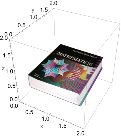
When constructing a volume from an array of data, by default the first three dimensions correspond to slices, rows, and columns of the 3D image, respectively. Slices are enumerated from top to bottom, rows from back to front, and columns from left to right.
A way to remember this is to think about placing a book in the 3D space. Pages of the book correspond to image slices (going from top to bottom) and data corresponding to each page (image slice) is arranged so that rows run from back to front and read from left to right.
Reshape the created list into a three-cube structure and create an Image3D object:
The Graphics3D primitive Raster3D displays the slices from bottom to top, and the rows of each slice are displayed from front to back:
Index Coordinates
For 3D images, similarly to 2D images, there is more than one coordinate system in use. The coordinate system used for embedding data arrays in 3D space is the same as the Wolfram Language's part specification.
The Wolfram Language commands that operate on both images and data arrays adhere to the index coordinate system. In 3D, these commands first list parameters that refer to the vertical slice coordinate going from top to bottom, then list the back-to-front row coordinate and then the left-to-right column coordinate.
Image Coordinates
The second coordinate system is not intrinsic to the data, but attached to the embedding space. The continuous image coordinate system, like the Graphics3D coordinate system, has its origin in the bottom-left front corner of an image with an  coordinate extending from left to right, a
  coordinate running from front to back, and a
  coordinate running from bottom to top. The image domain covers the 3D-interval
  ×
× ×
× .
.
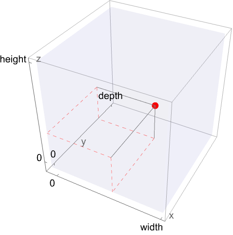
Image processing commands that are not applicable to arbitrary arrays render their results in standard image coordinates. These standard image coordinates can readily be used in Graphics3D primitives.