Image Processing
| Image Creation and Representation | Image Processing by Point Operations |
| Coordinate Systems | Image Processing by Area Operations |
| Basic Image Manipulation |
The Wolfram Language provides built-in support for both programmatic and interactive image processing, fully integrated with the Wolfram Language's powerful mathematical and algorithmic capabilities. You can create and import images, manipulate them with built-in functions, apply linear and nonlinear filters, and visualize them in any number of ways.
Images can be created from numerical arrays, from Wolfram Language graphics via cut-and-paste methods, and from external sources via Import.
| Image[data] | raster image with pixel values given by data |
| Import["file"] | import data from a file |
| CurrentImage[] | capture an image from a camera or other device |
The simplest way to create an image object is to wrap Image around a matrix of real values ranging from 0 to 1.
Another way is to copy and paste or drag and drop an image from some other application. You can use Import to obtain an image from a file on the local file system or any accessible remote location.
This imports an image from the Wolfram Language documentation directory ExampleData:
| ImageDimensions[image] | give the pixel dimensions of the raster associated with image |
| ImageAspectRatio[image] | give the ratio of height to width of image |
| ImageChannels[image] | give the number of channels present in the data for image |
| ImageColorSpace[image] | give the color space associated with image |
| ImageType[image] | give the type of values used for each pixel element in image |
| ImageQ[image] | |
| Options[symbol] | give the list of default options assigned to a symbol |
| ImageData[image] | the array of pixel values in image |
The image's array of pixel values can be easily extracted using the function ImageData. By default, the function returns real values, but you can ask for a specific type using the optional "type" argument.
In the case of multichannel images, the raw pixel data is represented by a 3D array arranged in one of two possible ways as determined by the option Interleaving.
With the default setting Interleaving->True, the data is organized as a 2D array of lists of color values, a triplet in the common case of images in RGB color space.
The option setting Interleaving->False can be used to store and retrieve the raw data as a list of matrices, one for each of the color channels.
A multichannel image can be split into a list of single-channel images and, conversely, a multichannel image can be created from any number of single-channel images.
Several image processing commands require or return positions in the image domain. To specify pixel positions, a coordinate system is required. Note that there is more than one coordinate system in use. This tutorial distinguishes between index coordinates and image coordinates.
Index Coordinates
Images are arrays of pixel data, and these arrays have row and column indices as inherent coordinates. Consequently, the Wolfram Language's part specification extends naturally as a discrete coordinate system to images.
Part specifications given by row and column indices are well-defined. However, the spatial embedding of an array is ambiguous.
Image renders the rows of an array from top to bottom:
The orientation of column and row coordinates depends on the spatial embedding. The first coordinate enumerating rows runs vertically, pointing up in the case of Raster and down in the case of Image. The second coordinate enumerating columns runs horizontally from left to right.


Wolfram Language commands that operate on both images and data arrays adhere to the index coordinate system. These commands first list parameters that refer to the vertical row-coordinate and then list parameters that refer to the horizontal column-coordinate.
Image Coordinates
The second coordinate system is not intrinsic to the data but attached to the embedding space. The continuous image coordinate system, like the graphics coordinate system, has its origin in the bottom-left corner of an image with an  coordinate extending from left to right and a
  coordinate running upward. The image domain covers the 2D-interval
  ×
× .
.

Image pixels are covered by intervals between successive integer coordinate values. Thus, noninteger coordinates refer unambiguously to a single pixel. Integer coordinates located on pixel boundaries, however, take all immediate pixel neighbors into account, either by selecting all neighboring pixels or by taking their average color value.


Image processing commands that are not applicable to arbitrary arrays render their results in standard image coordinates. These standard image coordinates can readily be used in Graphics primitives.
ImageLines returns lines in standard image coordinates:
For an image of height  , the conversion between index coordinates
  and standard image coordinates
  is given by
A slightly modified version of the standard image coordinate system is the normalized image coordinate system, in which the image width  is scaled to 1.

At times, it is more convenient to use normalized coordinates to specify operations that are independent of image dimensions.
Another modified version of the standard image coordinate system is the pixel-aligned coordinate system. The origin of this coordinate system is shifted by  to the left and down with respect to the standard image coordinate system to align the integer coordinates with pixel centers.

| PixelValue[image,{x,y}] | give the pixel value of image at position {x,y} |
| PixelValuePositions[image,val] | return a list of pixel positions in image that match the value val |
| ReplacePixelValue[image,{xp,yp}->val] | change the pixel values at pixel position {xp,yp} in image to val |
Consider the image manipulation operations that change the image dimensions by cropping or padding. These operations serve a variety of useful purposes. Cropping allows you to create a new image from a selected portion of a larger one, while padding is typically used to extend an image at the borders to ensure uniform treatment of the border pixels in many image processing tasks.
| ImageTake[image,n] | give an image consisting of the first n rows of image |
| ImageCrop[image] | crop image by removing borders of uniform color |
| ImageTrim[image,{{x1,y1},…}] | trim image to include the specified {xi,yi} pixels |
| ImagePad[image,m] | pad image on all sides with m background pixels |
ImageCrop conveniently complements ImageTake. Instead of specifying the exact number of rows or columns to be extracted, it allows you to define the desired dimensions of the resulting image, namely, the number of rows or columns that are to be retained. By default, the cropping operation is centered, thus an equal number of rows and columns is deleted from the edges of the image.
While ImageCrop is primarily used to reduce the dimensions of the source image, it is frequently desirable to pad an image to increase its dimensions. All the most common padding methods are supported.
It is frequently necessary to change the dimensions of an image by resampling, or to reposition it in some manner. Functions that perform these basic geometric tasks are readily available.
| ImageResize[image,w] | give a resized version of image that is w pixels wide |
| Thumbnail[image] | give a thumbnail version of image |
| ImageRotate[image] | rotate image counterclockwise by 90° |
| ImageReflect[image] | reverse image by top-bottom mirror reflection |
Here, ImageResize is used to increase and diminish the size of the original image, respectively:
ImageRotate is another common spatial operation. It results in an image whose pixel positions are all rotated counterclockwise with respect to a pivot point centered on the image.
Several useful image processing tasks require nothing more than simple arithmetic operations between two images or an image and a constant. For example, you can change brightness by multiplying an image by a constant factor or by adding (subtracting) a constant to (from) an image. More interestingly, the difference of two images can be used to detect change and the product of two images can be used to hide or highlight regions in an image in a process called masking. For this purpose, three basic arithmetic functions are available.
| ImageAdd[image,x] | add an amount x to each channel value in image |
| ImageSubtract[image,x] | subtract a constant amount x from each channel value in image |
| ImageMultiply[image,x] | multiply each channel value in image by a factor x |
Point operations constitute a simple but important class of image processing operations. These operations change the luminance values of an image and therefore modify how an image appears when displayed. The terminology originates from the fact that point operations take single pixels as inputs. This can be expressed as
where  is a grayscale transformation that specifies the mapping between the input image
  and the result
  , and
, and  ,
,  denotes the row, column index of the pixel. Point operations are a one-to-one mapping between the original (input) and modified (output) images according to some function defining the transformation T.
Contrast Modification
Contrast modifying point operations frequently encountered in image processing include negation (grayscale or color), gamma correction, which is a power-law transformation, and linear or nonlinear contrast stretching.
| Lighter[image,
…
] | give a lighter version of an image |
| Darker[image,
…
] | give a darker version of an image |
| ColorNegate[image] | give the negative of image, in which all colors have been negated |
| ImageAdjust[image] | adjust the levels in image, rescaling them to cover the range 0 to 1 |
| ImageApply[f,image] | apply f to the list of channel values for each pixel in image |
One of the simplest examples of a point transformation is negation. For a grayscale image f, the transformation is defined by
It is applied to every pixel in the source image. In the case of multichannel images, the same transformation is applied to each color value of every pixel.
The function ImageAdjust can be used to perform most of the commonly needed contrast stretching and power-law transformations, while ImageApply enables you to realize any desired point transformation whatsoever.
As an example of a nonlinear contrast stretching operation, consider the following transformation called sigma scaling. Assuming the default range of 0 to 1, the transformation is defined by
Image binarization is the operation of converting a multilevel image into a binary image. In a binary image, each pixel value is represented by a single binary digit. In its simplest form, binarization, also called thresholding, is a point-based operation that assigns the value of 0 or 1 to each pixel of an image based on a comparison with some global threshold value t.
Thresholding is an attractive early processing step because it leads to significant reduction in data storage and results in binary images that are simpler to analyze. Binary images permit the use of powerful morphological operators for shape and structure-based analysis of image content. Binarization is also a form of image segmentation, as it divides an image into distinct regions.
| Binarize[image] | create a binary image from image |
| ColorQuantize[image,n] | give an approximation to image that uses only n distinct colors |
Color images are first converted to grayscale prior to thresholding. If the threshold value is not explicitly given, an optimal value is calculated using one of several well-known methods.
Here ImageApply is used to return a color image in which each individual channel is binarized, resulting in a maximum of eight distinct colors:
Color Conversion
Supported color spaces include: RGB (red, green and blue), CMYK (cyan, magenta, yellow and black), HSB (hue, saturation and brightness), grayscale and device-independent spaces such as Lab.
In practice, the RGB (red, green, blue) color scheme is the most frequently used color representation. The three so-called primary colors are combined (added) in various proportions to produce a composite, full-color image. The RGB color model is universally used in color monitors, video recorders, and cameras. Also, the human visual system is tuned to perceive color as a variable combination of these primary colors. The primary colors added in equal amounts produce the secondary colors of light: cyan (C), magenta (M), and yellow (Y). These are the primary pigment colors used in the printing industry and thus the relevance of the CMY color model. For image processing applications it is often useful to separate the color information from luminance. The HSB (hue, saturation, brightness) model has this property. Hue represents the dominant color as seen by an observer, saturation refers to the amount of dilution of the color with white light, and brightness defines the average luminance. The luminance component may, therefore, be processed independently of the image's color information.
| ColorConvert[expr, colspace] | convert color specifications in expr to refer to the color space represented by colspace |
Note that the RGB->Grayscale transformation uses the weighting coefficients recommended for U.S. broadcast television (NTSC) and later incorporated into the CCIR 601 standard for digital video.
Image Histogram
An important concept common to many image enhancement operations is that of a histogram, which is simply a count (or relative frequency, if normalized) of the gray levels in the image. Analysis of the histogram gives useful information about image contrast. Image histograms are important in many areas of image processing, most notably compression, segmentation, and thresholding.
| ImageLevels[image] | give a list of pixel values and counts for each channel in image |
| ImageHistogram[image] | plot a histogram of the pixel levels for each channel in image |
Most useful image processing operators are area based. Area-based operations calculate a new pixel value based on the values in a local, typically small, neighborhood. This is usually implemented through a linear or nonlinear filtering operation with a finite-sized operator (i.e., a filter). Without loss of generality, consider a centered and symmetric 3×3 neighborhood of the image pixel at position  , with value
 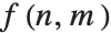 . A general area-based transformation can be expressed as
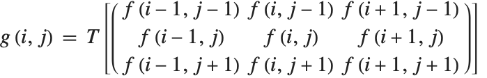
where  is the output image resulting from applying transformation
  to the 3×3 centered neighborhoods of all the pixels in input image
  . It should be noted that the spatial dimensions and geometry of the neighborhood are generally determined by the needs of the application. Examples of image processing region-based operations include noise reduction, edge detection, edge sharpening, image enhancement, and segmentation.
Linear and Nonlinear Filtering
Linear image filtering using convolution is one the most common methods of processing images. To achieve a desired result you must specify an appropriate filter. Tasks such as smoothing, sharpening, edge finding, and zooming are typical examples of image processing tasks that have convolution-based implementations. Other tasks, such as noise removal, for example, are better accomplished using nonlinear processing techniques.
| ImageFilter[f,image,r] | apply f to the range r of each pixel in each channel of image |
| ImageConvolve[image,ker] | give the convolution of image with kernel ker |
The more general (but slower) ImageFilter function can be used in cases when traditional linear filtering is not possible and the desired operation is not implemented by any of the built-in filtering functions.
A large number of linear and nonlinear operators are available as built-in functions. Here is a partial listing.
| Blur[image] | give a blurred version of image |
| Sharpen[image] | give a sharpened version of image |
| MeanFilter[image,r] | replace every value by the mean value in its range r |
| GaussianFilter[image,r] | convolve with a Gaussian kernel of pixel radius r |
| MedianFilter[image,r] | replace every value by the median in its range r |
| MinFilter[image,r] | replace every value by the minimum in its range r |
| CommonestFilter[image,r] | replace each pixel with the most common pixel value in its range r |
One of the more common applications of linear filtering in image processing has been in the computation of approximations of discrete derivatives and consequently edge detection. The well-known methods of Prewitt, Sobel, and Canny are all essentially based on the calculation of two orthogonal derivatives at each point in an image and the gradient magnitude.
As a second example, consider the task of removing the impulsive noise, which is called salt noise due to its visual appearance, from an image. This is a classic example contrasting the different outcomes resulting from a linear moving-average and a nonlinear moving-median calculation.
Morphological Processing
Mathematical morphology provides an approach to the processing of digital images that is based on the spatial structure of objects in a scene. In binary morphology, unlike linear and nonlinear operators discussed so far, morphological operators modify the shape of pixel groupings instead of their amplitude. However, in analogy with these operators, binary morphological operators may be implemented using convolution-like algorithms with the fundamental operations of addition and multiplication replaced by logical OR and AND.
| Dilation[image,r] | give the dilation with respect to a range-r square |
| Erosion[image,r] | give the erosion with respect to a range-r square |
This shows the dilation (left) and erosion (right), of a binary image (center) using a 5x5 uniform structuring element:
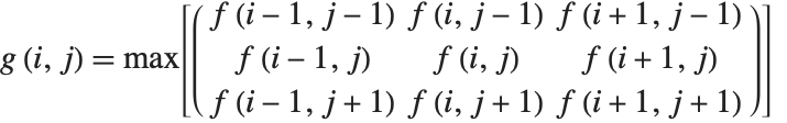
The definitions of binary morphology extend naturally to the domain of grayscale images with Boolean AND and OR becoming pointwise minimum and maximum operators, respectively. For a uniform, zero-valued structuring element, the dilation of an image  reduces to the following simple form:
This shows the dilation (left) and erosion (right), of the example color image (center) using a 5x5 uniform structuring element:
These operators can be used in combinations using a single structuring element or a list of such elements to perform many useful image processing tasks. A partial listing includes thinning, thickening, edge and corner detection, and background normalization.
| GeodesicDilation[marker,mask] | give the fixed point of the geodesic dilation of the image marker constrained by the image mask |
| GeodesicErosion[marker,mask] | give the fixed point of the geodesic erosion of the image marker constrained by the image mask |
| DistanceTransform[image] | give the distance transform of image, in which the value of each pixel is replaced by its distance to the nearest background pixel |
| MorphologicalComponents[image] | give an array in which each pixel of image is replaced by an integer index representing the connected foreground image component in which the pixel lies |
An important category of morphological algorithms, called morphological reconstruction, is based on repeated application of dilation (or erosion) to a marker image, while the result of each step is constrained by a second image, the mask. The process ends when a fixed point is reached. Interestingly, many image processing tasks have a natural formulation in terms of reconstruction. Peak and valley detection, hole filling, region flooding, and hysteresis threshold are just a few examples. The latter, also known as a double threshold, is an integral part of the widely used Canny edge detector. Pixels falling below the low threshold are rejected, pixels above the high threshold are accepted, while pixels in the intermediate range are accepted only if they are "connected" to the high threshold pixels. Connectivity may be established using a variety of algorithms, but reconstruction gives an effective and very simple solution.