3.13.1 ConvertDataTo2D

Command structure of ConvertDataTo2D.

All Analog Insydes functions which return numerical data, e. g. ACAnalysis, NoiseAnalysis, NDAESolve, or ReadSimulationData use the data format described in Section 3.7.1. This format is suitable for representing one, two, and multi-dimensional numerical data. As standard Mathematica graphic functions do not support the multi-dimensional Analog Insydes data format, ConvertDataTo2D converts the data such that it can be plotted with standard Mathematica graphic functions such as Plot3D.

The input data must be two-dimensional data as described in Section 3.7.1, for example:

Data format for two-dimensional numerical simulation data.

{

{

V$1 -> InterpolatingFunction[{{t1, t2}}, <>],

,

SweepParameters -> {VIN -> v1}

},

,

{

V$1 -> InterpolatingFunction[{{t1, t2}}, <>],

,

SweepParameters -> {VIN -> v2}

}

}

The data will then be converted to a set of two-dimensional interpolating functions:

Converted data format.

{

V$1 -> InterpolatingFunction[{{v1, v2}, {t1, t2}}, <>],

,

}

Please note the order of the parameters for the two-dimensional interpolating function. The interpolation order is set to {1, 1}.

See also: Section 3.7.1, Section 3.7.2.

Examples

Load Analog Insydes.

In[1]:= <<AnalogInsydes`

Read the simulation data with ReadSimulationData.

In[2]:= data = ReadSimulationData[
"AnalogInsydes/DemoFiles/Multivibrator.txt",
Simulator -> "PSpice"]

Out[2]=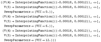

Convert it into two-dimensional interpolating functions.

In[3]:= data2d = ConvertDataTo2D[data]

Out[3]=

Display simulation result with Plot3D.

In[4]:= Plot3D[
Evaluate[("V(4)"[VCC, IC]-"V(5)"[VCC, IC]) /. data2d],
{IC, -0.00018, 0.00011}, {VCC, 0., 12.},
BoxRatios -> {1., 1., 1.},
AxesLabel -> {"IC", "VCC", "V(4)-V(5)"}]

Out[4]=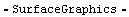