8. Inverse Dynamics

Overview

This chapter covers MechanicalSystems basic dynamic modeling capabilities for fully constrained models. If mass properties are defined for the bodies in a model, Mech can calculate the inertial loads on the model and the resulting reaction forces. Because the inertial loads are a function of the velocity and acceleration of the bodies, a model must have some dependence on time in order to have nonzero inertial loads. The forces that result from an inverse dynamic analysis are represented in the same manner as those of a static analysis, in the form of Lagrange multipliers (generalized forces). The free response dynamics of underconstrained systems is covered in Chapter 10.

8.1 Inertia Properties

In order for any inertial loads to exist in a mechanism model, the bodies of the mechanism must have nonzero inertia properties, mass and inertia. The inertia properties of the bodies in a model are defined in Mech body objects, and then added to the current model with the SetBodies command.

8.1.1 Body Options

Mech body objects are used to define specific properties of a body in a mechanism model. Properties are defined with options to the Body function.

The body object builder.

Two of the options for Body that are used for basic kinematic models are PointList and InitialGuess, which are discussed in Section 2.1. The remaining three options for Body are used to define the inertia properties of a body.

2D

2D inertia property options for Body.

3D

3D inertia property options for Body.

Executing the Body function does not, in itself, have any affect on the current Mech model. The returned SysBody data objects must be added to the model with the SetBodies command.

The body object processing function.

8.1.2 Examples

To use the 2D example mechanism of Section 1.2 in a dynamic analysis, inertia properties would be added with body objects and the SetBodies function. The crankshaft-piston mechanism used three Modeler2D bodies: the ground, crankshaft, and piston.

This loads the Modeler2D package.

In[1]:=

Names are defined for each of the bodies in the model.

In[2]:=

For this example, it is assumed that the constraints of the crankshaft-piston model have already been defined as they were in Section 1.2.
There is no use in adding inertia properties to the ground body, as it cannot move, and therefore can sustain no inertial loads. The inertia properties of the crankshaft and piston are defined and added to the model.

Here are the mass and inertia properties for the crankshaft and piston.

In[5]:=

The inertia properties must be incorporated into the model.

In[7]:=

Because the default setting for all options for Body is Automatic, which leaves the current values of properties unchanged, a single inertia property can be changed without affecting the rest of the model. An example is changing the location of the centroid of the piston without changing any other body properties.

This moves the centroid of the piston only.

In[8]:=

Each of the inertia property options for Body can be interrogated to find the current settings of a body property.

Inertia property functions.

Here is the mass of the crankshaft.

In[9]:=

Out[9]=

8.1.3 Compound Inertia Properties

The centroidal inertia properties of a 3D body in a mechanism model must be determined before the dynamic reaction forces in a model can be found. For complex 3D bodies, the values of the moments and products of inertia can be quite difficult to determine manually. This problem is alleviated by the availability of 3D solid modeling systems that can generally calculate the inertia properties of any solid body that they are capable of modeling.
If the inertia properties of a body must be found manually, the body can be subdivided into several elementary geometrical components such as spheres, cylinders, or plates. Modeler3D provides several functions to aid in manipulating the inertia properties of a body or multiple bodies. These functions can make the task of determining the inertia properties of a slightly complex body more manageable.

Utilities for manipulating 3D inertia properties.

Inertia Transformations

The following example takes the inertia properties of a triangular plate that are calculated in a noncentroidal reference frame and convert them to a centroidal frame. The plate is an isosceles right triangle with two one-unit sides.

Triangular plate

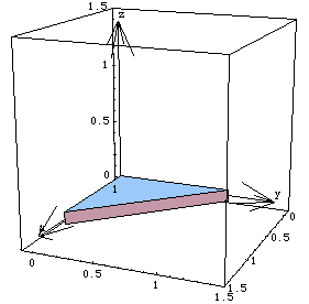
The inertia properties of the plate, in the shown reference frame, can be integrated directly or found in an engineering or mathematics handbook.

Here are the basic inertia properties of the plate.

In[10]:=

Out[10]=

iyy is known by symmetry.

In[11]:=

In[12]:=

Out[12]=

In[13]:=

Out[13]=

iyz and izx are zero because the plate has zero thickness.

In[14]:=

The location of the centroid of the plate can also be found by direct integration, knowing that the mass of the plate is 1/2 because the density of the plate is one unit mass per unit area.

Here are the mass and centroid location.

In[15]:=

In[16]:=

Out[16]=

This loads the Modeler3D package.

In[17]:=

To use the ParallelAxis function to transform noncentroidal inertia properties into a centroidal reference frame, instead of vice versa, the vector from the centroid to the origin of the noncentroidal frame is specified in the centroidal reference frame coordinates, and a negative mass is specified. Note that the sign of the centroid vector is irrelevant, but it must be given in the correct reference frame if there is any relative rotation between the frames.
ParallelAxis returns the centroidal inertias {Ixx, Iyy, ...} that are reduced in magnitude relative to the noncentroidal properties.

Here are the centroidal inertia properties of the plate.

In[18]:=

Out[18]=

The principal axes of inertia of the plate can be found with the PrincipalAxes function. Note that the list of the three principal axes of inertia forms the rotation matrix from the local reference frame of the inertia properties to the principal reference frame.

Here are the principal inertias and axes of the plate.

In[19]:=

Out[19]=

This rotates the original inertia matrix into the principal frame.

In[20]:=

Out[20]=

Composite Bodies

The CompositeInertia function is used to add the inertia properties of several bodies together and return the centroidal inertia properties of their superset. In the following example, the inertia properties of the triangular plate are added to the inertia properties of a cylinder that is attached to the plate and rotated through a 30-degree angle about the local x axis, as shown below. The radius of the cylinder is 0.25 and the length is 1 unit. The bottom surface of the cylinder is coplanar with the local x axis of the plate.

A composite body

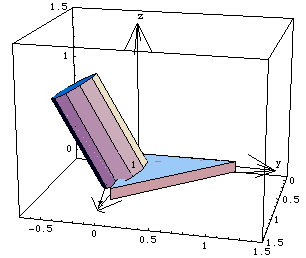
The centroidal inertia properties of a cylinder in an axial reference frame can be found in an engineering manual. These properties have been determined and are given in the following example.

Here are the inertia properties of the cylinder.

In[21]:=

Out[22]=

In[23]:=

Out[23]=

In[24]:=

Out[24]=

CompositeInertia can now be used to combine the inertia properties of the plate and the cylinder into one set of centroidal inertia properties. Note that the optional rotation argument is used for the cylinder since the reference frame in which its inertia properties were calculated was not aligned with the local reference frame.

Here are the inertia properties of the combined thin plate and cylinder.

In[25]:=

Out[25]=

2D Inertia Functions

Modeler2D also provides two inertia transformation functions that parallel those in Modeler3D, although the calculations they perform are trivial by comparison.

Utilities for manipulating 2D inertia properties.

Undocumented Graphics Generation

8.2 Kinematic and Dynamic Solutions

This section describes the function of Mech's inverse dynamics solution block. Inverse dynamics allows the dynamic reaction forces in a fully kinematically constrained model to be found. The motion of such a model is completely defined by the kinematics of the model, only the reaction forces that result from the constrained motion are found through inverse dynamics. To find the free response of a model with one or more degrees of dynamic freedom, consult Chapter 10.

8.2.1 Dynamics Options

Once the kinematic constraints and the inertia properties of a body have been defined, the dynamic forces in a mechanism can be determined. The Solution option to SolveMech is used to tell Mech to calculate the generalized reaction forces in the model and to include the forces due to inertia.

An option for SolveMech.

The purpose of the Kinematic setting is to allow for velocity-dependent loading, such as damping, while still not including the dynamic loading. Note that using the Static setting does not necessarily produce an error in a model that has velocity-dependent loading, because Static sets the velocities to zero. This condition may result in an incidental error, however, if the velocity-dependent terms happen to blow up at zero velocity.
The Dynamic setting calculates the mechanism accelerations and then adds the inertial loads due to the acceleration of each body to the model's applied load vector before calculating the generalized reaction forces. Note that the Dynamic setting must be used to include the centrifugal forces, even though they depend on velocity and not acceleration.

8.2.2 3D Example Mechanism

A Modeler3D example model is developed to demonstrate a simple gyroscopic inertial loading condition. The model is a flywheel with an angular velocity vector with a changing direction.
The model consists of only one moving body, the flywheel. The flywheel spins about an axis that is attached to the ground at one point. The axis of rotation of the flywheel is then rotated about another nonparallel axis affixed to the ground. Thus, the direction of the axis of rotation of the flywheel changes with time.

This loads the Modeler3D package.

In[1]:=

Here is a graphic of the flywheel model.

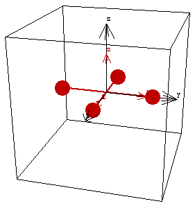
The Method -> Angular option is given to SetSymbols before building any other part of the flywheel model. This is done so that the angular velocity and angular acceleration of the flywheel is calculated directly, instead of being calculated in terms of derivatives of Euler parameters. Note that this is not a necessary step to obtain the dynamic forces.

This causes angular velocities to be calculated directly so that it won't be necessary to convert the Euler parameters into angular velocity.

In[2]:=

Inertia

The flywheel is modeled by four one-unit point masses, symmetrically placed about the axis of rotation. The Modeler3D CompositeInertia function can be used, trivially, to find the net inertia properties of the flywheel.

In[3]:=

Out[4]=

Bodies

One body object is defined for the flywheel model. The ground body does not have a body object because it has no inertia or required point definitions. The body object for the flywheel contains the inertia properties and the locations of each of the four point masses.

Names are defined for each of the body numbers in the model.

In[6]:=

Here is the body object for the flywheel.

In[8]:=

Constraints

Three constraints, two of which are functionally dependent on time, are required to model the flywheel mechanism.
A Spherical3 constraint places the center of the flywheel at the global origin.
A Parallel2 constraint forces the axis of rotation of the flywheel to be parallel with a specified vector on the ground body. The direction of the axis vector on the ground body is explicitly a function of time T. This constraint effectively causes the axis of rotation of the flywheel to change direction with time.
A ProjectedAngle1 constraint rotates the flywheel about its axis. Note the choice of the vector that was used on the ground body. The vector in the Y direction on the ground body is always normal to the axis of rotation of the flywheel. If a vector in the X direction was chosen instead, the constraint would become singular at T = 0.25. Note also that the flywheel is spinning 10 times more rapidly about its symmetry axis than its axis is rotating with respect to the ground.

Here are the constraint objects for the flywheel.

In[9]:=

Runtime

Because of the presence of T in the constraints, the model can be run through its intended range of motion by varying T directly with the SolveMech command.

Now run the model at T = 0.02.

In[10]:=

Out[10]=

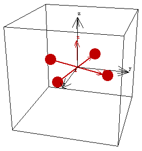
Here is the flywheel at T = 0.02.

8.2.3 Inertial Loading

No forces are applied to the model with SetLoads because only the inertial loading of the flywheel is being considered. All of the inertia properties have already been defined, so all that must be done to find the dynamic solution is to request it of SolveMech with the solution option.

The dynamic solution at T = 0.

In[11]:=

Out[11]=

The angular velocity and acceleration of the flywheel can be read directly from the solution rules returned by SolveMech, or Modeler3D output functions can be used. Note that the angular acceleration is orthogonal to the angular velocity.

Here are the angular velocity and acceleration of the flywheel.

In[12]:=

Out[12]=

The moment that is applied to the flywheel to enforce the specified rotation is the reaction force to constraint 2, the constraint that controls the direction of the axis of the flywheel.
Note that the reaction to constraint 3 is zero. No moment is required to spin the flywheel about its primary axis, only to change the direction of the axis.

Here are the moments that are applied to the flywheel by the constraints.

In[13]:=

Out[13]=

In[14]:=

Out[14]=

As the position of the flywheel is advanced in time, the components of the angular velocity change, and the components of the angular acceleration and the applied moment follow.

This calculates the dynamic solution at T = 0.01.

In[15]:=

Here are the angular velocity and acceleration.

In[16]:=

Out[16]=

Here is the applied moment.

In[17]:=

Out[17]=

Undocumented Graphics Generation

8.3 Friction and Damping

This section demonstrates various techniques of applying friction and damping forces to a mechanism model with MechanicalSystems.

8.3.1 Types of Friction

Loads that can be applied to a Mech model fall into four basic categories with considerable overlap between them.
An applied load is a load in which the magnitude and/or direction depends on the configuration of the model, on time, or is constant. Applied loads may or may not be conservative. Loads of this type are discussed throughout Chapter 7.
A damping load is a nonconservative load in which the magnitude and/or direction depends on the velocity of the model. These loads are modeled by giving an expression for the load magnitude or direction that is functionally dependent on velocity terms, and then using the Kinematic or Dynamic option settings for SolveMech.
A frictional load is a nonconservative load in which the magnitude and/or direction depends on the reaction forces applied by the constraints. These loads are modeled by giving an expression for the load magnitude or direction that is functionally dependent on the Lagrange multipliers, usually by using the Reaction function to find the reaction force at a constraint.
An inertial load is a load in which the magnitude and/or direction depends on the linear and angular acceleration and angular velocity of bodies in the model. Inertial loads are applied to the model automatically by specifying inertia properties for each body, and then using the Dynamic option setting for SolveMech, as discussed in Section 8.2.

Damping

Damping loads are usually applied to a model in a relatively simple manner. To apply linear damping to a point on a moving body, a force is applied to the body that is inversely proportional to the velocity of the point. The magnitude of the force is proportional to the magnitude of the velocity of the point (relative to whatever the point is in contact with) and the direction vector of the force is opposite the velocity vector of the point.

This loads the Modeler3D package.

In[1]:=

The velocity of a point.

The following example shows how damping with a damping constant of 4.0 would be applied to a point at local coordinates {1, 0, 0} on body 2 in a 3D model.

Here is an example of an applied damping load.

In[2]:=

Out[2]=

The line of action of the force passes through Point[2, {1,0,0}], which is not dependent on velocity, and points in the direction of the velocity of the point. The negation of the velocity vector causes the applied force to oppose the motion of the point, and the Magnitude -> Relative setting causes the magnitude of the force to be 4.0 times the magnitude of the velocity vector, instead of a constant magnitude of 4.0.
To model point damping that occurs at an interface between two moving bodies, the velocity of the point to which damping is applied must be known relative to the body that the point is in contact with. The Mech RelativeVelocity function returns this vector quantity.

The velocity of a point relative to another body.

The following example shows how damping that exists between body 2 and body 3, with a damping constant of 4.0, would be applied to body 2 at local coordinates {0, 1, 0} in a 3D model.

Here is a load object that models point damping between two bodies.

In[3]:=

Out[3]=

Note that the preceding example only applies the frictional force to body 2. An equal and opposite force should also be applied to body 3.

Friction

A Coulombic friction load is functionally dependent on reaction forces in the model. Such a load is usually applied by making the magnitude of the load a function of reaction forces by using the Mech Reaction function.

The reaction load from a constraint.

Coulombic friction forces may also be dependent on velocity terms to establish the direction of the frictional force.
The following example shows how the friction of a point sliding on a plane might be modeled. The model uses a PointOnPlane1 constraint to place a point on body 2 in contact with a plane on body 3, and a coefficient of friction between the point and the plane is 0.3. The frictional force would be modeled in the general case by using the velocity vector of the point, relative to the plane, to define the direction of the force, and the reaction to the constraint times the coefficient of friction to define the magnitude.
The second constraint in the following SetConstraints call is just a dummy constraint to fill out the needed 12 degrees of freedom.

Here is a dummy SetConstraints call with a PointOnPlane1 constraint.

In[4]:=

The optional second argument of Force is used here to apply a force to body 2 and an equal and opposite force to body 3.

Here is a general method for modeling Coulombic friction on a PointOnPlane1 constraint. The coefficient of friction is 0.3.

In[5]:=

Out[5]=

8.3.2 Damping Example

To demonstrate the application of damping to a Mech model, a 2D model of a simple four-bar linkage is developed. The model consists of three moving bodies: the drive bar, the driven bar, and the center bar. The kinematic input to the model is the rotation of the drive bar.
Damping is first applied to the model at a point on the center bar that traces out an eccentric path in the 2D plane. Coulombic friction is then applied to the rotational axis of the drive bar.

This loads the Modeler2D package.

In[6]:=

Here is the four-bar mechanism, with a moving point locus.

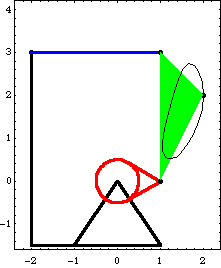
Bodies

Four body objects are required for the four-bar model. Each bar is attached to another bar at its local origin and at a point at the other end of the bar on the local X or Y axis.

Names are defined for each of the body numbers in the model.

In[7]:=

Here are the body objects for the four-bar model.

In[13]:=

The body properties are incorporated into the current model.

In[17]:=

Constraints

Five constraints, one of which is a driving constraint, are required to model the four-bar mechanism. A RotationLock1 constraint is used as a driving constraint to rotate the drive bar. Four Revolute2 constraints model the four pivot points in the four-bar mechanism.

Here are the constraint objects for the four-bar model.

In[18]:=

The constraints are incorporated into the current model.

In[23]:=

Damping Load

A damping force is applied to point 2 on the center bar relative to the ground. The direction of the frictional force opposes the global velocity of point 2, and the coefficient of damping is 5.0.

Here is a damping load.

In[24]:=

The load is incorporated into the current model.

In[25]:=

Runtime

Because of the presence of T in the driving constraint cs[1], the model can be run through its intended range of motion by varying T directly with the SolveMech command. The numerical value of T specifies the angle of rotation of the drive bar in revolutions.

Now run the model at T = 0.3.

In[26]:=

Out[26]=

Here is the four-bar model at T = 0.3.

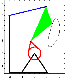
Because the loading in this model is dependent on velocity terms, the Solution -> Kinematic option must be used with SolveMech to solve for the reaction forces. If Solution -> Static were used, SolveMech would assume that all velocities were zero, thus, the applied damping would have zero magnitude and zero reactions would result.

Here is the solution, including the generalized reaction forces.

In[27]:=

Out[27]=

The reaction moment at the rotational driver is the moment required to rotate the drive bar.

In[28]:=

Out[28]=

Here is the reaction force at the drive bar axis.

In[29]:=

Out[29]=

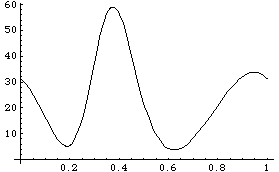
Plots

To generate a plot of the torque required to turn the drive bar, the four-bar model is run from T = 0 to T = 1 in 21 steps, a full turn of the drive bar, while requesting that SolveMech interpolate the results.

This generates an interpolated solution set and returns one part of the solution.

In[30]:=

Out[30]=

Here is an explicit expression for the drive torque.

In[31]:=

Out[31]=

Here is a plot of the drive torque as a function of time.

In[32]:=

Out[32]=

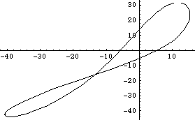
A parametric plot of the x-y reaction at the axis of the drive bar can be easily created. The plot ranges only from T = 0 to T = 0.95 so the start and end points are apparent.

Here is the drive arm axis reaction vector.

In[33]:=

Out[33]=

Here is a parametric plot of the drive arm axis reaction vector.

In[34]:=

Out[34]=

Friction Load

A very simple Coulombic friction load is applied to the rotational axis of the drive bar, with respect to the ground. The load is a pure moment resisting the direction of motion, the magnitude of which is proportional to the magnitude of the reaction vector at the drive bar axis. A coefficient of friction of 0.5 is assumed and is applied to a journal bearing with radius 0.4.

Here is a simple Coulombic friction load.

In[35]:=

The load is added to the current model.

In[36]:=

More Plots

This generates another interpolated solution set.

In[37]:=

The drive torque function that was developed earlier can be plotted again with the new solution rules. Note that the required drive torque is slightly higher.

Here is a plot of the drive torque with friction at the drivebar axis.

In[38]:=

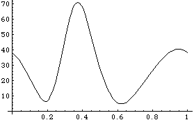
Out[38]=

8.3.3 Friction Example

To demonstrate the application of Coulombic friction to a Mech mechanism model, a 2D model of a slider on an inclined ramp is developed. The model consists of one moving body, the slider.
As the slider is pushed along its track on the ground body, it travels along the initial horizontal part of the track until the tip of the slider encounters the upward turn of the track. The tip then progresses up the inclined ramp while the heel of the slider stays on the horizontal section. Coulombic friction is modeled at the two sliding interfaces at the tip and the heel of the slider. The Modeler2D TimeSwitch function is used to switch between the different friction forces as the tip of the slider passes from one section of the ramp to the next.

This loads the Modeler2D package.

In[39]:=

Here is a graphic of the 2D slider-ramp model.

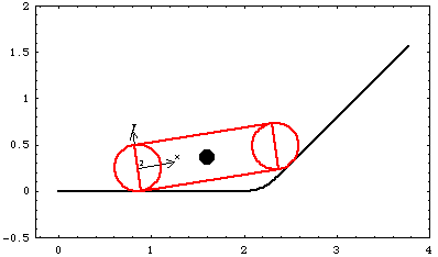
Bodies

Two body objects are defined for the slider-ramp model.

Note that points 3, 4, and 5 on the ramp are defined as functions of two user-defined variables radius and incline, so that the radius at the curve of the ramp and the angle of the incline can be changed easily.
Because a gravitational force will be applied to the slider, the mass and centroid location are defined in the slider's body object.

Names are defined for each of the bodies in the model.

In[40]:=

Here are the body objects for the slider-ramp.

In[42]:=

In[44]:=

In[45]:=

The body properties are added to the current model.

In[46]:=

Constraints

Three constraints, one of which is a driving constraint, are required to model the slider-ramp mechanism.

The value of the initial switch time determined by inspection is 0.5. However, the value of the second switch time is more difficult to determine analytically, so it is left as the symbol swtime and the FindSwitchTime function is used to find a numeric value.

Here are the constraint objects for the slider-ramp model.

In[47]:=

Here, the constraints are added to the current model.

In[51]:=

Runtime

Before the model can be run the undefined symbols, incline, radius, and swtime, must be defined. $MechVariables returns the names of any symbols that have been recognized as being part of the current model.

Here is a Mech utility.

In[52]:=

Out[52]=

The embedded symbols are explicitly defined.

In[53]:=

Now the model is run at T = 0.65.

In[56]:=

Out[56]=

Here is the slider-ramp model at T = 0.65.

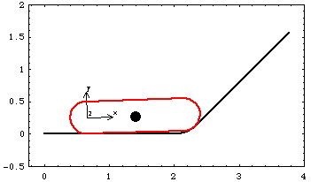
Switch Time

Now the exact value of swtime can be found with FindSwitchTime. Because the slider passes tangentially from the curved section of the ramp onto the inclined section (which implies that there is no discontinuity in the velocity of the slider at the transition), the TangentConstraint option must be used with FindSwitchTime. This option tells FindSwitchTime to look for the point of velocity equality instead of just location equality.

Find switch time 2 in constraint 3.

In[57]:=

Out[57]=

Loads

The goal of this example is to determine the force required to push the slider around the curved section of the ramp and up the incline, with gravity pulling down on the slider, and friction between the slider and the ramp at both ends.
First, gravity is applied without any friction forces. A plot of the force required to push the slider is made from a list of solutions returned by SolveMech.

Here is a gravitational load.

In[58]:=

The model is run from T = 0.0 to 1.8.

In[59]:=

Out[59]=

Here is a plot of the driving force.

In[60]:=

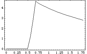
Out[60]=

Now a friction force is added to the left end of the slider. This is fairly straightforward, as the line of action of the force is constant throughout the motion of the slider. The force is applied to the slider and the line of action is along the surface of the ramp. The magnitude of the force is equal to the coefficient of friction times the normal force at the left end of the slider, which is the Y reaction to constraint 2.

Here is the left end friction load. The symbol cf is the coefficient of friction.

In[61]:=

Now a friction force is added to the right end of the slider. This is rather complicated, as the line of action of the friction force changes as the slider passes from one section of the ramp to another.
The friction force is applied to the slider, but the line of action is along the surface of the ramp. On the two flat sections of the ramp, the friction force is applied in the same manner as the force on the left end of the slider. However, the line of action of the force around the curve on the ramp has to be developed directly with vector algebra.
Although the line of action changes as the slider moves through the different stages of the ramp, the magnitude of the normal force is always equal to the coefficient of friction times the magnitude of the reaction force of constraint 3, even though constraint 3 is changing from one constraint type to another.
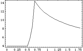
TimeSwitch is used to switch between the forces in exactly the same manner as it is used to switch constraints, without the constraint number argument. Since the forcing functions switch at the same times as the constraints, the same switch times can be used.

Here is the right end friction load

In[63]:=

All of the defined loads are added here to the current model.

In[65]:=

SolveMech is called with intermediate times in between the beginning and end times that are explicitly included in the points in time that are solved for. This ensures that a data point is included exactly at the peak of the force plot.

The model is now run through a range of 30 points in time, including the two switch times.

In[66]:=

Out[66]=

Here is a plot of the driving force.

In[67]:=

Out[67]=

Undocumented Graphics Generation

Four-Bar

Slider-Ramp