7. Loads and Reactions

Overview

This chapter describes how MechanicalSystems is used to apply forces and moments to a mechanism model, and how the resulting reaction forces in the constraints are resolved. Mech uses a Lagrange multiplier method to resolve the applied and reaction loads on each body, and solves for a generalized force associated with each constraint. These generalized forces can then be converted back into the force and moment applied by a selected constraint to each body in the model with a standard Mech output function.

7.1 Load Objects

Load objects are used to define the forces and moments that are to be applied to a Mech model. All Mech load functions return load objects with the head SysLoad. To apply the loads to the mechanism model, the load objects are passed to the SetLoads function. This syntax is analogous to the way that constraint objects are passed to SetConstraints to incorporate them into the model.

7.1.1 2D Load Functions

The Modeler2D load functions are used to specify forces and moments applied to specific bodies in the mechanism model. In general, moments are specified by magnitude, and forces are specified by magnitude and line of action.
By using Modeler2D axis objects to define the line of action, a force can be applied to a point attached to any body in the mechanism, and the direction of the force can be a global or local vector, or a line from one body to another. The magnitude of a force or moment applied to a static model can be a constant, or it can be a function of location or velocity-dependent variables or even a function of the reaction forces at specified constraints. An applied load that is a function of constraint reaction forces is often used to model friction.

2D load functions.

An option for Force.

Modeler2D load objects are typically used in a similar manner to Modeler2D constraint objects. They are defined prior to adding them to the model and then passed to SetLoads. Some examples of valid load objects follow.

This loads the Modeler2D package.

In[1]:=

Here is a moment of magnitude 4 applied to the crank.

In[2]:=

Out[4]=

Here is a moment applied to the crank with magnitude equal to twice the rotation angle of the crank.

In[5]:=

Here is a force applied to the crank passing through point {1,1} on the crank and pointing in the global X direction, with magnitude equal to k times the distance from the point of application to the global origin.

In[6]:=

The Gravity function needs to know the mass and the location of the centroid of each body to apply the gravitational force. These properties are defined with the Mass and Centroid options for the Modeler2D Body function, and added to the model with SetBodies. See Section 8.1.

7.1.2 3D Load Functions

The Modeler3D load functions are used to specify forces and moments applied to specific bodies in the mechanism model. In general, moments are specified by magnitude and direction, and forces are specified by magnitude and line of action.
By using Modeler3D axis objects to define the line of action of forces, and Modeler3D vector objects to define the direction of moments, a force can be applied to a point attached to any body in the mechanism, and the direction of a force or moment can be a global or local vector, a line from one body to another, or even the normal of a plane. The magnitude of a force or moment applied to a static model can be a constant, or it can be a function of location or velocity-dependent variables or even a function of the reaction forces at particular constraints.

3D load functions.

An option for Force and Moment.

Modeler3D load objects are typically used in a similar manner to Modeler3D constraint objects, they are defined prior to adding them to the model and then passed to SetLoads. Some examples of valid load objects follow.

This loads the Modeler3D package.

In[7]:=

Here is a moment of magnitude 4 and a direction vector in the global Z direction applied to the crank.

In[8]:=

Out[10]=

Here is a moment applied to the crank with magnitude equal to twice the rotation angle of the crank, relative to the global reference frame, and direction vector on the local x axis.

In[11]:=

Here is a force applied to the crank passing through point {1, 1, 0} on the crank and pointing in the global X direction, with magnitude equal to k times the distance from the point of application to the global origin.

In[12]:=

The Gravity function needs to know the mass and the location of the centroid of each body to apply the gravitational force. These properties are defined with the Mass and Centroid options for the Modeler3D Body function, and added to the model with SetBodies. See Section 8.1.

7.1.3 Generalized Load Function

The Load function is analogous to the Mech Constraint function. Load allows the user to specify an algebraic expression to be added directly to the model's load vector, just as Constraint allows an algebraic constraint to be added to the constraint list.

The generalized load function.

The Load function is typically used only when special generalized coordinates have been added to the model, and it is necessary to apply a load directly to those coordinates. Load basically allows expressions to be added directly to a model's load vector. Using Load to apply a load to a model's Cartesian coordinates is equivalent to applying a force or moment to a body in the model.

Here are Load and Force objects that are functionally equivalent.

In[13]:=

Out[13]=

Out[14]=

In 3D models, the sym argument to Load has a special caveat: if the Angular solution method was specified with SetSymbols, loads cannot be directly applied to the Euler parameters, because the load vector is formulated in terms of angular velocity. However, loads can be applied directly to the angular velocity coordinates, which is equivalent to applying a pure moment.

Here are Load and Moment objects that are functionally equivalent, when the SetSymbols settings are as specified.

In[15]:=

Out[16]=

Out[17]=

7.2 Static Solutions

Load objects are applied to the current model with the SetLoads function. The actual load vector developed by SetLoads is not returned to the user, rather it is stored in several variables in the `Private` context of the Mech packages. The use of load objects and SetLoads in Mech is analogous to the use of constraint objects and SetConstraints.
Mech uses a Lagrange multiplier method to resolve the constraint reaction forces in a mechanism model. There is one Lagrange multiplier named 1, 2, and so on for each degree of freedom in the model. Thus, when Mech solves a loaded model what is returned to the user are the numerical values of the Lagrange multipliers. The Lagrange multipliers are actually the generalized forces related to a set of generalized coordinates in which each coordinate corresponds to the magnitude of the violation of a kinematic constraint.
While the numerical values of the Lagrange multipliers are not directly very useful, they are converted into the reaction forces and moments that are applied by the constraints to each body in the model with the Reaction function. This is discussed in Section 7.3.

7.2.1 2D Example Mechanism

To demonstrate the use of Mech's static force solution method a 2D model is developed that is subject to applied loads. A 3D model would be treated in the same manner as 2D with regard to the application of forces. The model is a simple ladder sliding down a wall consisting of one moving body, the ladder.
The input to the mechanism is to push the bottom of the ladder across the horizontal floor, in either direction. The ladder is constrained such that the bottom of the ladder must contact the floor and the top of the ladder must contact the vertical wall.

This loads the Modeler2D package.

In[1]:=

Here is a graphic of the 2D ladder-on-wall model.

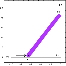
Bodies

Two body objects are defined for the ladder-on-wall model.

Names are defined for each of the body numbers in the model.

In[2]:=

Here are the body objects for the ladder-on-wall model.

In[4]:=

SetBodies incorporates the body properties into the current model.

In[6]:=

Constraints

Three constraints, one of which is a driving constraint, are required to model the ladder-on-wall. The top and bottom tips of the ladder, which slide on the wall and floor, each have a small radius.

Here are the constraint objects for the ladder-on-wall model.

In[7]:=

SetConstraints incorporates the constraint objects into the current model.

In[10]:=

7.2.2 Applying Loads

SetLoads is the core function for applying loads to a Mech model. SetLoads takes load objects that represent the physical loads applied to the model and builds them into a global load vector that represents the total force and moment applied at the origin of each body in the model.

The load application function.

Mech uses a Lagrange multiplier method to resolve the static and dynamic forces on a model, which will be discussed further in Section 7.3. It is usually not necessary to specify initial guesses for the Lagrange multipliers, because the equations of motion are linear in the Lagrange multipliers unless friction forces are applied. If initial guesses are needed, they can be specified with the LambdaGuess option for SetLoads.

An option for SetLoads.

Because forces and moments are additive quantities, it is not necessary to apply all of the loads to the model simultaneously. With the AddLoads option, loads can be applied to the model sequentially.

An option for SetLoads.

Loads for the Model

Three loads are defined for the model developed in Section 7.2.1.

Here are the load objects for the ladder-on-wall model.

In[11]:=

Out[13]=

Initially, only the two Force objects are applied. SetLoads incorporates the loads into the model.

In[14]:=

By using the AddLoads option for SetLoads, additional loads can be applied to the model at any time. Thus, the Moment can simply be added to the current loading.

This adds the Moment object to the ladder-on-wall model.

In[15]:=

Mech load objects can contain dependencies on other dependent variables. For example, to model the force applied by a linear spring, it is necessary to have the magnitude of the force be a function of the distance between two points.
The Force of an extension spring with a free length of 2 units and a spring constraint k attached between the top of the ladder and the top of the wall could be modeled as follows.

Here is a spring force.

In[16]:=

7.2.3 Running the Loaded Model

Because of the presence of T in the driving constraint cs[1], the model can be run through its intended range of motion by varying T directly with the SolveMech command. The numerical value of T specifies the distance between the bottom of the ladder and the wall.
Although loads have been added to the model, the SolveMech default option setting Solution -> Location solves only for the location variables.

Now run the model at T = 7.5.

In[17]:=

Out[17]=

Mech must be told to solve for the static forces in the model with the Solution option for SolveMech.

An option for SolveMech.

The Solution -> Static option causes SolveMech to resolve the forces applied to the model into Lagrange multipliers.

Now run the model at T = 8.5.

In[18]:=

Out[18]=

Here is the ladder-on-wall image at T = 8.5.

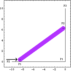
The numeric values of the Lagrange multipliers returned by SolveMech are not directly very useful, unless one has a very good understanding of the exact form of the constraints. However, the set of Lagrange multipliers associated with a mechanism model completely determines all of the reaction forces in the constraints in the model. To find the actual reaction forces and moments at a specific constraint it is necessary to use the Mech Reaction function, which is described in Section 7.3.

Undocumented Graphics Generation

7.3 Resultant Forces

This section describes the usage of the two Mech functions that are used to convert the Lagrange multipliers into reaction forces on specific bodies in a model, Reaction and Loads.

7.3.1 2D Example Mechanism

To demonstrate the use of Mech's Reaction function, the 2D ladder-on-wall model that was developed in Section 7.2 is used. The bodies and constraints of the model are redefined here in abbreviated form.

The following loads the Modeler2D package and completely defines the ladder-on-wall model.

In[1]:=

In[4]:=

In[5]:=

The model is run to prove that it works.

In[6]:=

Out[6]=

7.3.2 Reaction

The Reaction function is used to convert the Lagrange multipliers that are returned by SolveMech into specific reaction forces and moments that are applied to each body by the constraints in the mechanism model.

The function for finding constraint reaction forces.

An option for Reaction.

To demonstrate the use of Reaction, loads are applied to the ladder-on-wall model that was redefined in Section 7.3.1.

Here are the load objects for the ladder-on-wall model.

In[7]:=

Only the first two loads are added to the model initially; the other load will be added later. The model can then be run with the Solution -> Static option to solve for the Lagrange multipliers.

Load 1 and load 2 are applied to the current model.

In[10]:=

Now run the model at T = 6.0.

In[11]:=

Out[11]=

Because the Reaction function references constraints by number, names are given to each of the constraints for clarity.

Names are defined for each of the constraints in the model.

In[12]:=

The horizontal force at the bottom of the ladder that is required to hold the ladder in its current position is the reaction to constraint 1, the driving constraint. Note that the Y force and the moment sustained by the driving constraint are both zero, and always will be, because the driving constraint (RelativeX1) does not constrain motion in the Y or directions, therefore, it cannot sustain any load in those directions.

Here is the reaction to the driver.

In[17]:=

Out[17]=

For the ladder to be in equilibrium, the force at the driver must be balanced by the force against the wall. Note that the Reaction function, like all other Mech output functions, returns a symbolic expression in terms of dependent variables.

Here is the reaction against the wall.

In[18]:=

Out[18]=

Out[19]=

Note that if a different point is chosen about which to calculate the reaction, only the moment is changed. A reaction force is not a function of the point about which the reaction is calculated, therefore, the choice of a calculation point never affects the force, only the moment.

Here is the reaction against the wall calculated about a point on the ground.

In[20]:=

Out[20]=

Since there is no friction in this model, the sum of all of the vertical forces is applied to the floor.

Here is the reaction against the floor.

In[21]:=

Out[21]=

When the applied moment, load 3, is added to the model, it shows up as added reaction force against the driver and the wall.

The moment that was previously defined is added to the model.

In[22]:=

Here is the reaction against the wall.

In[23]:=

Out[23]=

7.3.3 Loads

The actual load vector that is generated by SetLoads can be directly accessed with Loads. Loads can be very useful for debugging a model because it is often possible to read the load expressions directly and relate them to the function of the model.

The load inspection function.

An option for Loads.

If the Coordinates option is not specified, Loads returns forces that are generalized to the current velocity coordinate system. Since velocity in the current model is represented by {Xnd, Ynd, nd} the returned loads are {Fx, Fy, M}, calculated about the local origin. Consider the 2D ladder-on-wall model of Section 7.3.2. Loads can be used to find the total load applied to the ladder resolved into a force applied to the origin of the ladder, and a moment.

Here is the total load applied to the ladder.

In[24]:=

Out[24]=

Out[25]=

In all cases, the sum of the applied, reaction, and dynamic loads on any body must be zero. Since there are no dynamic loads in this model, the total reaction loads on all constraints must be equal to the total applied loads.

Here is the total reaction load applied by the constraints to the ladder.

In[26]:=

Out[26]=

Out[27]=

The dynamic, or inertial, loads on the ladder are identically zero because there are no masses or moments of inertia defined. If there were, the dynamic loads would be functions of the model's acceleration variables, X3dd, Y3dd, and so on.

Here are the inertial loads on the ladder.

In[28]:=

Out[28]=

Note that the numerical sum of the loads is zero, but the algebraic terms are quite different. This basically shows part of the system of equations that was solved by SolveMech when the numeric values of the Lagrange multipliers were found.

7.4 Multistage Loads

This section demonstrates how to use StageSwitch and TimeSwitch in the context of a loaded mechanism model. The use of StageSwitch and TimeSwitch in a kinematic model is covered in Chapter 5. In general, switching forces on and off is treated in the same way as switching constraints on and off.

7.4.1 Stage and Time Switches

StageSwitch

The Mech StageSwitch function is used for loads in the same manner as it is used for constraints, with one important difference. Because loads are cumulative, StageSwitch can apply more than one of the switched loads at a time, or no loads at all.

The multistage mechanism load-switching function.

Unlike most built-in Mathematica switching functions, StageSwitch does evaluate its arguments immediately. This means that test functions such as SameQ cannot be used because SameQ evaluates to True or False immediately, without waiting for some future condition to change and make it True or False in the context of the mechanism model. StageSwitch will fail if any of the test expressions fail to return True or False at runtime.
Each of the loads supplied to the StageSwitch must be a Mech load object with the head SysLoad, or a nested list of load objects.

Example

This loads the Modeler2D package.

In[1]:=

The following example shows how a StageSwitch might be used to model a force that is either a constant force in one direction or a function of T in another direction. Which force is applied is determined by the value of the user-defined symbol whichload.

Here is a valid StageSwitch load object.

In[2]:=

Out[5]=

TimeSwitch

The TimeSwitch function is also used to apply loads in much the same way it is used to apply constraints. The primary difference is that the load object TimeSwitch may have a leading time, before which no load is applied, and a trailing time, after which no load is applied.

The time-dependent, load switching function.

Each of the loads supplied to the TimeSwitch must be a Mech load object or a nested list of load objects.

Example

The following example shows how a TimeSwitch might be used to model a force applied to the slider that is to remain constraint in magnitude until the value of time reaches 2.0, at which time the force begins to increase linearly with time.

Here is a valid TimeSwitch load object.

In[6]:=

In[8]:=

Out[8]=

7.4.2 2D Example Mechanism

To demonstrate the use of Mech's StageSwitch function, a 2D model is developed that is subject to a variable applied load. The model is a simple piston-pump that has a nonlinear compression function applied to the piston.
The input to the model is to rotate the crankshaft. The pressure on the piston increases slowly but nonlinearly until near the end of its stroke, at which time the pressure decreases very rapidly back to zero. The pressure then remains at zero through the return stroke of the piston.

Here is the 2D piston-pump graphic.

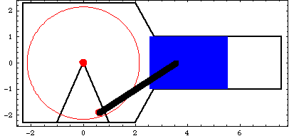
Constraints

Four constraints, one of which is a driving constraint, are required to model the piston-pump. Body objects are not defined for this model. The coordinates of the local points are simply entered directly in the point and axis objects in the constraints.

Names are defined for each of the bodies in the model.

In[9]:=

Here are the constraint objects for the model.

In[12]:=

Here is a reasonable initial guess for the piston.

In[17]:=

Loads

Only one load is applied to the piston-pump model, but this one load will be a two-stage StageSwitch load. Since the piston is initially at the top of its stroke and proceeds toward the bottom, there is no load on the piston for the first half turn of crank rotation. The two segments of the StageSwitch load are defined as follows.

Here are the two forces on the piston.

In[18]:=

The StageSwitch load must switch between f1 and f2 at the proper time. This is done by testing the value of the X coordinate of the piston X3 and the angular coordinate of the crank 2.

Here is the StageSwitch load object for the pump.

In[20]:=

Out[20]=

The loads are incorporated into the model.

In[21]:=

Running the Model

The loaded model can now be run with the Solution -> Static option for SolveMech. Note that all of the loads are zero at T = 0.1 because the force is turned off.

Now run the model at T = 0.1.

In[22]:=

Out[22]=

Here is the piston-pump model at T = 0.1.

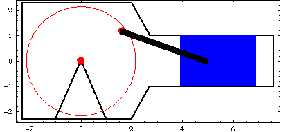
By creating a large table of solution points, plots can be made of various forces, moments, and reactions in the model using ListPlot.

Here is a list of 81 solutions.

In[23]:=

The Loads function returns the total load on the piston.

In[24]:=

Out[24]=

The force on the piston can be plotted as a function of piston travel.

In[25]:=

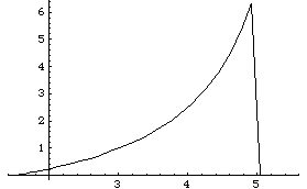
Out[25]=

The reaction forces at the constraints can be found with the Reaction function. Constraint 4 is the RotationLock1 driving constraint, so its reaction is the moment applied to the crank. Constraint 1 is the Revolute2 constraint that positions the crank axis, so its reactions are the X and Y forces supporting the crank axis.

Here is the moment required to rotate the crank.

In[26]:=

Out[26]=

Here is the reaction at the crank as a function of time.

In[27]:=

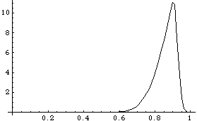
Out[27]=

Because ListPlot is not able to plot two lists simultaneously, Mathematica graphics primitives are used directly to plot the X and Y reactions.

Here are the X and Y reaction forces at the crank axis as a function of time.

In[28]:=

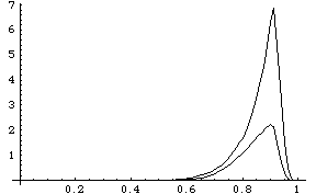
Out[28]=

Undocumented Graphics Generation