EquationTrekker Package

Basic Use	Defining Your Own Trek Generator
Parameters	Interactive Controls
Poincaré Sections

This package provides an interactive tool for investigating the solutions of differential equations as well as other types of equations that have solutions that can be viewed as paths or trajectories.

The Wolfram Language provides a general tool, NDSolve, for finding numerical solutions of differential equations. The ability to simply specify differentiation equations in mathematical form gives a great deal of convenience over Fortran and C++ solver packages. However, for low-dimensional systems, an additional level of interactivity can be achieved with a graphical user interface. EquationTrekker allows you to give the equation, optionally with parameters, and then it opens a window that allows you to specify initial conditions simply by using the mouse.

This loads the package.

Basic Use

EquationTrekker[eqns,y,{x,x_min,x_max},opts]
	open a graphical interface for specifying initial conditions and showing the resulting numerical solutions to the ordinary differential equations eqns for the function y with the independent variable x in the range x_min to x_max

Choosing initial conditions for differential equations using a graphical interface.

It is appropriate to start with a very simple example to demonstrate how EquationTrekker operates. Enter the following.

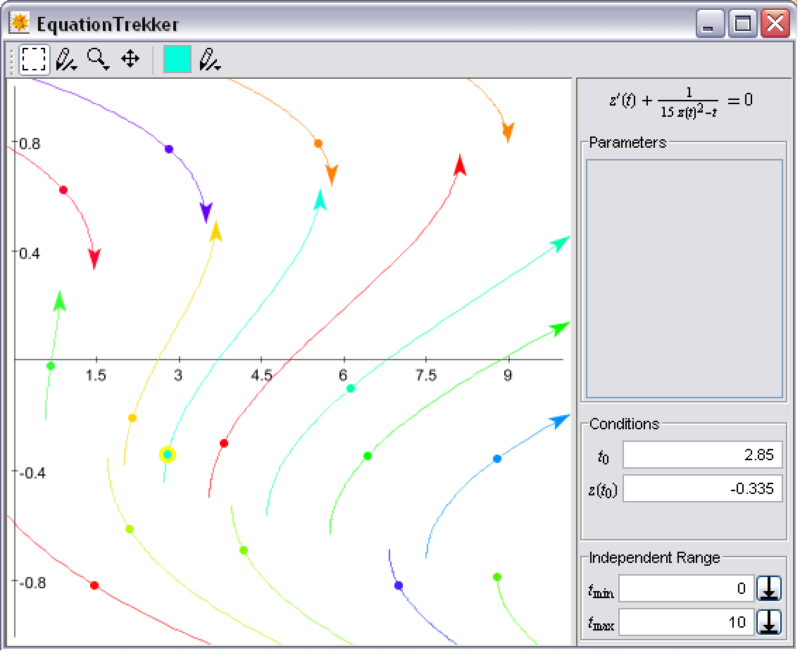
It brings up a separate window like the one shown here (starting with a blank canvas).

The curves shown, which will be called "treks", are the solutions (shown in the versus phase plane) with initial conditions through the points displayed as dots. By default, is taken to be zero, and the trek is shown for the extent of the range (x_min, x_max) given in the command, in this example, to . To choose an initial condition, all you have to do is position the cursor and right-click. The trek will be shown as soon as it can be computed by NDSolve, which, for this example, is within the blink of an eye! If you hold the right button down and drag the cursor, the solution will be updated in real time as you drag. The currently selected trek is indicated by the larger yellow circle. You can see from the screenshot that there are numerous controls and values that can be set. Each of these will be described once the Wolfram Language interface has been demonstrated.

This starts EquationTrekker for the simple harmonic oscillator. When you enter this command, a window like the screenshot earlier will open. The window is running modally, which means that until you close the window, the kernel is controlled through the window. When you close the window, a list is returned and kernel control reverts to the notebook.

The returned list has only two elements, an EquationTrekkerState object and a graphic. The graphic displays the treks that were generated while the window was open. The EquationTrekkerState object contains all of the information required to reopen the window with the same treks as it had when it was closed, allowing you to save interesting cases to be explored later. Its output forms are abbreviated, showing the equations, variables, and a list of the treks generated, each of which displays only its initial condition.

EquationTrekkerState[eqns,y,{x,x_min,x_max},treks,<data>]
	a data object that can be reused to open an EquationTrekker window with a list treks representing treks that were generated; the data is not shown in output forms by default
Trek[condition,<data>]	a data object that represents a single trek; in output forms, only the values of condition which were chosen to generate the trek are shown
EquationTrekker[state]	open up an EquationTrekker window with the treks saved in the EquationTrekkerState object state

EquationTrekker state objects.

This reopens the EquationTrekker window in the state it had been in when the window was closed to generate the above results.

To get the result just shown, once the window was opened, the Del key was pressed, deleting the selected trek, and then the window was closed, generating a new state.

Because of the need to choose conditions in two dimensions, EquationTrekker is limited to one or two first-order equations or a single second-order equation. A system of two first-order equations looks very much like the previous example; in fact, second-order equations are converted to first-order equations. A single first-order equation is somewhat different in that when you click a point, you are in effect choosing the starting value of the independent variable, whereas with two equations, the value of the independent variable is taken to be zero (this can be modified through the graphical interface).

For example, when EquationTrekker is invoked, a window looking like this screenshot is generated.

Parameters

The ability to specify multiple initial conditions is remarkably useful, but EquationTrekker goes a step further in allowing you to investigate the solutions of differential equations. Using the TrekParameters option, you can give the equation with symbolic parameters, which are controlled through the EquationTrekker window interface.

Including a nonlinear term makes a somewhat more interesting equation to investigate than the simple harmonic oscillator.

This opens an EquationTrekker window for a nonlinear perturbation of the simple harmonic oscillator. Sliders are included in the window, which allow you to control the values of α and ω.

When you move the sliders (or modify the text values and press Enter), the new solutions are calculated immediately and the window is updated, allowing you to rapidly get an idea of how the parameters affect the solutions of the equation.

This opens up the same window. The results shown are arrived at by changing the parameter values in the window to

and

. It is apparent that a new separatrix has formed.

You can specify the range of possible values as well as the starting value when you specify a parameter.

name->value	parameter name will start with value and have range [0,2 value] (or [-1,1] if value is 0)
name->{value,{v_min,v_max}}	parameter name will start with value and have range [v_min,v_max]

Parameter specifications.

This allows the parameter ω to be specified in the range [0,20]. For higher frequencies, a somewhat complicated set of orbits and separatrices exists. The result shown was chosen by using

It would have been much more difficult to find these features without the interactivity.

You might notice that if you run this example and generate quite a few treks as shown earlier, it may take a while for the window to update when you do a parameter change. This is not surprising, since NDSolve has to recompute each of the solutions over again, and the rapidly varying nonlinear term leads to a more difficult numerical problem to solve.

Poincaré Sections

The default behavior of EquationTrekker is to show a straightforward plot of the solution parametrized by the independent variable. However, there are situations where such plots can get very confusing, particularly for non-autonomous equations (for which there is explicit dependence on the independent variable).

A good example of this is Duffing's equation, a nonlinear model for vibrations of a driven clamped beam.

This shows an example of treks generated by Duffing's equation.

The orbits cross one another and it is hard to get much of an idea of what to expect for nearby points.

A common technique for visualizing the overall change is to see how the solution is evolving over periods of the driving function. One way to think of this is to consider the three-dimensional space of (x, x^′, s), where s=Mod[ω t,2π]. In this case, the solutions lie within a torus. One way of visualizing the overall evolution of the solution is to see how it changes each time it has wrapped around the s axis, effectively looking at just a single cross section of the torus. This is one common case of a more general technique known as a Poincaré section. The induced map is referred to as the Poincaré map.

This allows you to generate a Poincaré section for Duffing's equation. The output shown was generated by picking two initial conditions. Note that the MaxSteps option is passed through to NDSolve: since it is computing the solution over quite a long time interval, it is appropriate to allow as many steps as are needed.

The image shows the so-called strange attractor for Duffing's equation, which demonstrates deterministic chaos for the starting parameter values. The attractive nature can be intuited from the way points from both initial conditions wind up on the same structure. Note that the minimum value of t for which points were shown was chosen to be quite large so that transients are allowed to decay. Often this is a good choice when investigating systems in this way.

To use the Poincaré section trek generator, you will have to define the properties of the section you wish to see with method options.

option name	default value
"SectionCondition"	None	an expression in the problem variables for which the section variables will be shown whenever the expression is zero
"SectionVariables"	None	a subset of two of the dependent variables (or their derivatives for second- and higher-order equations) which will be shown every time the section condition expression is zero
"FilterFunction"	None	a function to apply to the values of the section variables before plotting; this only affects the plot, not the selection of initial conditions

Method options for the PoincareSection trek generator.

It is required that you specify some value for both "SectionCondition" and "SectionVariables". Additionally, you can also pass to the generator any options of NDSolve you would like to be used in the computation.

When the value of "SectionCondition" is of the form Mod[ω t,T], where ω and T are constants (they can depend on trek parameters, just not on the independent variable t or any of the dependent variables), a special optimized code is used to handle this common case as in the preceding example.

This loads a package containing several examples of differential equations.

This gets the ABC (Arnold–Beltrami–Childress) flow system, which is used to model chaos in laminar flows of the three-dimensional Euler equations.

This starts EquationTrekker to compute a Poincaré section of the ABC flow. The section shows the variables

versus

when

. Before plotting,

and

are taken modulo

Defining Your Own Trek Generator

EquationTrekker has been set up in such a way that, with relatively little effort, you can define your own trek generator, which can then be used as a setting of the TrekGenerator option. The interface works through the construction of a trek generator object, which is initialized when EquationTrekker is started up and is expected to have methods defined with a particular argument structure.

InitializeGenerator[gname,spec,dvars,{ivar,iv_min,iv_max},opts]	initialize the trek generator with name gname with problem specification spec, dependent variables dvars, independent variable ivar with default range [iv_min,iv_max], and options opts
InitializeGenerator[gname,spec,vars,opts]	initialize the trek generator with name gname with problem specification spec, variables vars, and options opts; with this case, there is no independent variable, and the argument to EquationTrekker should be given as None

Initializing a trek generator.

InitializeGenerator[gname,…] should return an object of the form gname[args]. The arguments args of the object can be used to store any data that may be used by the trek generator. This data may be in any convenient form because it is private to the particular instance of the trek generator gname. Note: gname must be a Symbol.

It is recommended that you associate the rule for initializing a particular generator using InitializeGenerator with the generator name itself using TagSet (i.e., gname/:InitializeGenerator[gname,…]:=…). This avoids any possible problems with symbol protection and/or unintentionally affecting the initialization for other generators.

Once the trek generator object gobj=gname[args] has been defined, it is expected to have some methods defined. This is the mechanism through which EquationTrekker determines the display format and gets the generated points.

gobj@"Variables"[]	return a list of variables used by the trek generator; if there is an independent variable, it should be {ivar,dvars}
gobj@"Display"[]	return the equations or problem to show in the display area of the EquationTrekker window
gobj@"DisplayMode"[]	return the default display mode for treks, either "Line" or "Points"; this is just a default since the setting can be changed at any time through the EquationTrekker window interface
gobj@"FormatTrek"[iv0,X0,{iv_min,iv_max}]
	given the values of the independent iv0 and dependent X0 variables that specify starting values for a trek, return a descriptive form trek specification (note: even if the independent variable is not used, the argument will be present when this method is called)
gobj@"ChangeParameters"[prules]	return a new trek generator object that contains any new data that may be required to quickly generate points with modified parameter values given in the list of rules prules
gobj@"GenerateTrek"[X0,{iv0,iv_min,iv_max}]
	return the generated trek points for the trek starting from the point X0=(x0,y0) at independent variable value iv0; points should be generated over the independent variable range [iv_min,iv_max] (note: if there is no independent variable, this argument will still be present, though its value can be ignored; the points should be given a list of coordinates, {{x₁,y₁},{x₂,y₂},…}; if the process of generating points changes the arguments of gobj, this method can return a list {points,newgobj} containing a new trek generator object)

Methods for trek generator objects.

All the methods are necessary to have EquationTrekker display the modifiable items and problem specification in a reasonable way, but the essence of a particular trek generator will lie in how the "GenerateTrek" method is defined.

The ideas behind setting up a trek generator are best illustrated by some examples. The two examples that follow have been kept simple for the purposes of illustration. You can also see the definitions of the DifferentialEquationTrek and PoincareSection generators in the package file EquationTrekker.m.

Example: Nesting

This is a very simple generator that simply plots the result of applying NestList to a specified function. Even though the basic idea is simple, the idea of iteration is fundamental to most numerical methods, so a tremendous variety of methods and models can be visualized this way.

This declares the symbol Nesting to be in the EquationTrekker` context. If the EquationTrekker Package has been loaded, once this is entered, it is sufficient to just use Nesting to specify this symbol. See the note on contexts following this section for more detailed explanation.

InitializeGenerator is defined to be associated with Nesting. All it does is return an object with the function and variables in it. The function is repeated since, once the parameter is set, it will keep the original and the one transformed by the parameter rules.

Anything could be chosen as the appropriate thing to display. In this case, the obvious choice is the function being iterated.

Since the generator gives discrete iterations of function composition, it makes the most sense to show points, not lines, by default.

To keep the formatting simple, the method is defined to only show the starting point. Another option would be to use something like HoldForm[Nest[f,dv,n]], where n is the number of iterations.

When the parameters are changed, a new data object that saves the function transformed by the parameter rules is saved. This is the function that is actually given to NestList.

Finally, the all-important definition for generating points decides on the number of iterations (some argument checking on the values of iv0, ivmin, and ivmax would be appropriate here but has been left out for simplicity) and calls NestList.

This defines a function that defines a variant of Euler's method for the pendulum equation that conserves a Hamiltonian, which is within order h of the actual Hamiltonian for the pendulum equation.

This calls EquationTrekker to show the iterations of the function.

The level curves of the Hamiltonian conserved by the method are quite apparent from the graphic. By contrast, the usual explicit Euler method shows points that spiral outward since it is unconditionally unstable for the pendulum equation. If you vary h to be closer to zero, the curves become more and more like the actual orbits for the pendulum equation and the fuzziness near the separatrix disappears.

A Note on Contexts

The GUIKit application, which EquationTrekker is built from, modifies the contexts of input symbols that are in contexts not explicitly on the context path (given by $ContextPath) to avoid conflicts between invocations that may occur simultaneously.

This shows the value of the $ContextPath variable after the EquationTrekker Package has been loaded.

Symbols in Global` context will be given a private context. Typically, if you just enter a new symbol name, it will be created in the context, so definitions you make without consideration of context may not be recognized when you run EquationTrekker. To get around this problem, in the nesting example earlier, you can put Nesting into EquationTrekker` context, which was put on the context path when the EquationTrekker Package was originally loaded.

A tidier way to do it is to make a package that contains your trek generator definitions (e.g., Nesting`). When you load the package, its context will be put on the context path so the definitions will work properly. This method is shown in the next example.

Example: FindMinimum

A simple example that does not use an independent variable is a trek generator that simply shows the search points arrived at with FindMinimum, starting from a selected starting point.

This defines a package that sets up a trek generator based on FindMinimum.

The most significant difference between this generator and the one of the previous example is that it does not use an independent variable. This is reflected in InitializeGenerator in that the argument with independent variables is simply omitted. Aside from the "Variables" method, where only the used variables are returned, the arguments for the other methods have the same structure: even though the independent variables are not used, some (meaningless) values are passed anyway. This is done to optimize the overall operation of EquationTrekker.

The other thing worth noting in the previous definition is the way options are passed. FindMinimum options are selected with FilterRules and saved for use each time a trek is generated. These options come from options given to EquationTrekker when it is invoked.

This shows the search points for FindMinimum for a family of functions like the Rosenbrock function.

Interactive Controls

The graphical interface controls for EquationTrekker are generally self-explanatory. Following is a reference for the controls with a brief usage description.

The trek toolbar appears across the top of the EquationTrekker window:

The first four controls allow you to change the current mode. The last two allow you to select colors and display the current drawing mode.

icon	mode
	select treks mode	Mouse button selects treks. Multiple treks may be selected by dragging or using Shift+click. Once treks are selected, you may • Delete them by using the Del key. • Move their starting position(s) by dragging. • Change their color using the color well tool . Ctrl+click or right-click creates treks. Dragging allows you to interactively change the position of the newly created trek.
	create treks mode	Mouse button creates new treks. Ctrl+click or right-click selects treks. Dragging the create treks button opens a menu that allows you to toggle the default drawing mode between lines and points. The last item on the toolbar indicates the current drawing mode.
	zoom mode	In zoom mode, • Dragging the mouse shows a rectangle which will become the new range. The default behavior is to use a rectangle which preserves the aspect ratio of the current graph. Pressing the Ctrl key while dragging changes to a rectangle which can change the aspect ratio. • Shift+drag shows a rectangle that the edges of the current plot region will be mapped to (zoom out). • Ctrl+drag (right drag) pans. Dragging the Zoom Mode button opens a menu which allows you to select zoom to fit or scale to fit. Zoom to fit finds a plot range in which all the trajectories fit, preserving aspect ratio. Scale to fit finds the smallest plot range in which all the trajectories fit.
	pan mode	Mouse button pans selected point to center. Dragging pans interactively. Right-click or Ctrl+click zooms.

Modes chosen from the trek toolbar.

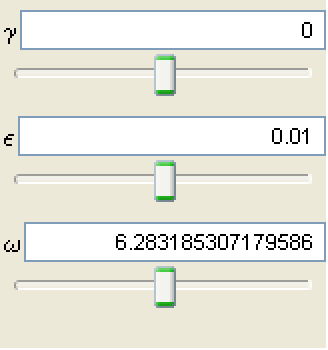
The parameter panel allows you to modify any parameters you have specified using the TrekParameters option.

Any parameter value can be modified either by using the slider or by typing the desired value into the text field and entering it.

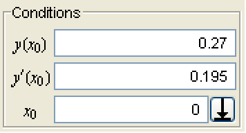
The conditions panel typically reflects the starting position and (if applicable) the starting independent variable value.

You can change any of the values by moving the trek position graphically or by typing in the desired position and entering it.
The

button allows you to change the default starting value of the independent variable for newly created treks.

When there is an independent variable, the independent range panel is displayed.

Entering values allows you to change the range of independent variable values for a selected trek. Using the

button allows you to change the default values for newly created treks.

Top