Heat Transfer
Introduction
This tutorial gives an introduction to modeling heat transfer. Equations and boundary conditions that are relevant for performing heat transfer analysis are derived and explained.
Heat transfer is a discipline of thermal engineering that is concerned with the movement of energy. The driving force behind a heat transfer are temperature differences. The temperature differences come about though different phenomena in the interior or on the boundary of the simulation domain and can be categorized into thermal conduction, thermal convection and thermal radiation. Combining all effects, the changes in a temperature field in a given region over time is then modeled with a heat equation.
The modeling process results in a partial differential equation (PDE) that can be solved with NDSolve. Furthermore, in this tutorial different types of heat sources are introduced as well as an overview of how various real world thermal interactions can be modeled with the available thermal boundary conditions.
The accuracy and the effectiveness of the heat transfer PDE model is validated in the separate notebook entitled Heat Transfer Verification Tests.
Extended examples of heat transfer modeling can be found in the Model Collection.
Many of the animations of the simulation results shown in this notebook are generated with a call to Rasterize. This is to reduce the disk space this notebook requires. The downside is that the visual quality of the animations will not be as crisp as without it. To obtain high quality graphics remove or comment out the call to Rasterize.
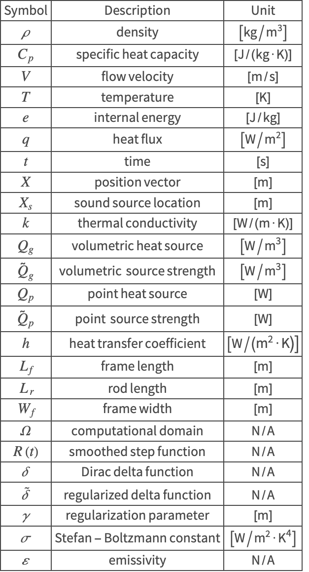
The symbols and corresponding units used throughout this tutorial are summarized in the Nomenclature section.
Heat Equation
Introduction to Heat Equation
The heat equation (1), which is derived from the law of energy conservation, is used for modeling time dependent heat flow within a thermally conductive medium:
The dependent variable in the heat equation is the temperature ![]() , which varies with time
, which varies with time ![]() and position
and position ![]() . The partial differential equation (PDE) model describes how thermal energy is transported over time in a medium with density
. The partial differential equation (PDE) model describes how thermal energy is transported over time in a medium with density ![]() and specific heat capacity
and specific heat capacity ![]() . The specific heat capacity is a material property that specifies the amount of heat energy that is needed to raise the temperature of a substance with unit mass by one degree Kelvin.
. The specific heat capacity is a material property that specifies the amount of heat energy that is needed to raise the temperature of a substance with unit mass by one degree Kelvin.
Beside the time derivative part the PDE is made up of several components. First and foremost there is a diffusive term: ![]() with a thermal conductivity
with a thermal conductivity ![]() . The thermal conductivity may very well depend on the temperature
. The thermal conductivity may very well depend on the temperature ![]() itself. This will then result in a nonlinear heat equation.
itself. This will then result in a nonlinear heat equation.
A second part is a convective term: ![]() with a flow velocity
with a flow velocity ![]() for modeling internal heat convection. This term is only present if the medium allows for an internal flow. If the simulation medium is a solid then this term is zero.
for modeling internal heat convection. This term is only present if the medium allows for an internal flow. If the simulation medium is a solid then this term is zero.
The term ![]() denotes a heat source within the domain, and is explained in the Source Types section.
denotes a heat source within the domain, and is explained in the Source Types section.
Heat Equation Derivation
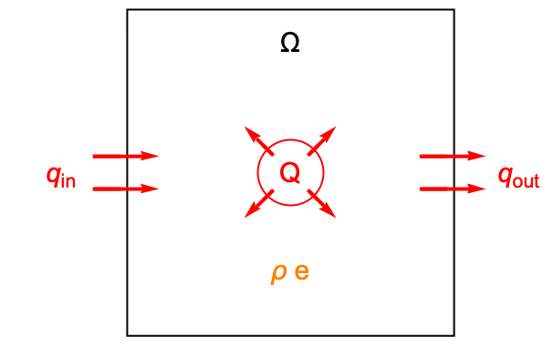
To derive the heat equation start from energy conservation. Consider balancing the energy generated within a unit volume domain ![]() with the energy flowing through the boundary of the domain.
with the energy flowing through the boundary of the domain.
In the above graphics, ![]() is the density and
is the density and ![]() is the internal energy per unit mass. The total energy within the control volume is then equal to the product
is the internal energy per unit mass. The total energy within the control volume is then equal to the product ![]() . The red circle in the middle represents a heat source
. The red circle in the middle represents a heat source ![]() , which denotes thermal energy that is generated inside the domain
, which denotes thermal energy that is generated inside the domain ![]() . The heat flux
. The heat flux ![]() represents the net energy that exits through the boundaries.
represents the net energy that exits through the boundaries.
The unit of the heat flux ![]() depends on the dimension of the boundary. In a 3D domain the boundary is represented by 2D surfaces, and the heat flux
depends on the dimension of the boundary. In a 3D domain the boundary is represented by 2D surfaces, and the heat flux ![]() has a unit of
has a unit of ![]() . In a 2D domain, however, the boundary has 1D lines, which makes the unit of
. In a 2D domain, however, the boundary has 1D lines, which makes the unit of ![]() become
become ![]() . In 1D the boundary is represented by a dimensionless point and the heat flux
. In 1D the boundary is represented by a dimensionless point and the heat flux ![]() has a unit of
has a unit of ![]() .
.
The energy balance within the domain ![]() can be described by the following equation:
can be described by the following equation:
That is, the change in the total energy ![]() is equal to the energy
is equal to the energy ![]() generated inside the domain minus the net energy that exits the domain
generated inside the domain minus the net energy that exits the domain ![]() .
.
Here the energy flux ![]() can be divided into two parts: a convection term
can be divided into two parts: a convection term ![]() and a diffusion term
and a diffusion term ![]() . The convection term denotes the energy transported by a possible flow inside the medium, and is in proportional to a flow velocity
. The convection term denotes the energy transported by a possible flow inside the medium, and is in proportional to a flow velocity ![]() :
:
If the heat transfer occurs in a solid medium, then, because a solid can not have an internal velocity field ![]() by definition, the convection term is set to
by definition, the convection term is set to ![]() .
.
The diffusion term represents the energy flux resulting from the energy gradient, and is proportional to its energy diffusivity ![]() :
:
For heat transfer modeling the diffusion term (2) is often expressed in the form of the temperature gradient ![]() instead, which is known as Flourier's law of heat conduction:
instead, which is known as Flourier's law of heat conduction:
Here the energy diffusivity ![]() is represented by the thermal conductivity
is represented by the thermal conductivity ![]() , and the minus sign indicates that the heat diffusion is in the direction of decreasing temperature.
, and the minus sign indicates that the heat diffusion is in the direction of decreasing temperature.
Note that the diffusive component is always present, regardless of the medium.
The principal property of the diffusion term is smoothing, this is explained in the section: The Smoothing Characteristic of the Diffusion Equation.
Inserting (3) and (4) into the energy balance equation (5) yields:
Note that the above equations hold for both continuous and discontinuous density/velocity fields. This is explained in more detail in the appendix Conservation Laws with Discontinuous PDE coefficients.
Since we consider a domain ![]() with a unit volume
with a unit volume ![]() , the total mass within the domain is then equal to:
, the total mass within the domain is then equal to: ![]() . Therefore, the term:
. Therefore, the term: ![]() on the left hand side can be interpreted as a mass conservation equation. Specifically, the time derivative part is understood as the accumulation (or loss) of mass in the domain
on the left hand side can be interpreted as a mass conservation equation. Specifically, the time derivative part is understood as the accumulation (or loss) of mass in the domain ![]() over time, while the divergence term part denotes the difference of the mass inflow versus outflow.
over time, while the divergence term part denotes the difference of the mass inflow versus outflow.
When there is no internal mass generation/destruction, the rate of the mass inflow is equal to the rate of the mass outflow plus the accumulation of mass within the domain ![]() . That is, the term
. That is, the term ![]() sums up to zero and can be removed from the equation (6) leading to:
sums up to zero and can be removed from the equation (6) leading to:
This leads to a restriction on the usage of the heat transfer model: Equation (7) and the resulting heat transfer PDEs (8) and (9) can not be used when the mass in the medium changes.
Since the internal energy ![]() depends on the temperature:
depends on the temperature: ![]() , equation (10) can be rewritten into the following form using the chain rule:
, equation (10) can be rewritten into the following form using the chain rule:
Here the term ![]() is also known as the specific heat capacity
is also known as the specific heat capacity ![]() , which denotes the ratio of the energy added to/removed from the domain to the resulting temperature change. With this definition equation (11) simplifies to the heat equation:
, which denotes the ratio of the energy added to/removed from the domain to the resulting temperature change. With this definition equation (11) simplifies to the heat equation:
The general heat equation describes the energy conservation within the domain ![]() , and can be used to solve for the temperature field
, and can be used to solve for the temperature field ![]() in a heat transfer model. Since it involves both a convective term and a diffusive term, the equation (12) is also called the convection-diffusion equation.
in a heat transfer model. Since it involves both a convective term and a diffusive term, the equation (12) is also called the convection-diffusion equation.
In a solid medium, however, the internal velocity field ![]() is set to zero and the governing PDE simplifies to a pure conductive heat equation:
is set to zero and the governing PDE simplifies to a pure conductive heat equation:
Note that the preceding heat equation (13) is written in a non-conservative form. That is, the ![]() term and with it the density
term and with it the density ![]() and the velocity
and the velocity ![]() are outside of the divergence operator. One could imagine that convective term inside the divergence operator. However, since both
are outside of the divergence operator. One could imagine that convective term inside the divergence operator. However, since both ![]() and
and ![]() might be space dependent, the general heat equation (14) cannot simply be transformed into a conservative form.
might be space dependent, the general heat equation (14) cannot simply be transformed into a conservative form.
The heat equation may also be expressed in cylindrical and spherical coordinates. Please refer to the appendix section "Special Cases of the Heat Equation" for detail explanation.
Heat Transfer Model Setup
Defining a function that represents the spatial terms of a heat transfer model in Cartesian coordinates will make the setup of a heat equation more convenient.
The inputs needed for an heat transfer model are
| the temperature variable | ||
| the spatial independent variables | ||
| a velocity field | ||
| the thermal conductivity | ||
| the density | ||
| the heat capacity | ||
| a heat source/sink |
Note that this model definition uses inactive PDE operators. "Numerical Solution of Partial Differential Equations" has several sections that explain the use of inactive operators.
Model Parameter Setup
The following model parameters are used for the examples in this notebook. These parameters define the simulation domain ![]() , the simulation end time
, the simulation end time ![]() and thermal properties of a medium.
and thermal properties of a medium.
In some examples we will be using a smoothed step function ![]() to prescribe a time profile for a transient parameter, for example the heat flux
to prescribe a time profile for a transient parameter, for example the heat flux ![]() or the surface temperature
or the surface temperature ![]() . The smoothed step function is defined as follows:
. The smoothed step function is defined as follows:
Here the minimum value and the maximum value the function ![]() can reach are denoted by
can reach are denoted by ![]() and
and ![]() . The location of the step is controlled by
. The location of the step is controlled by ![]() and the smoothed steepness is controlled by
and the smoothed steepness is controlled by ![]() .
.
Basic Heat Transfer Example
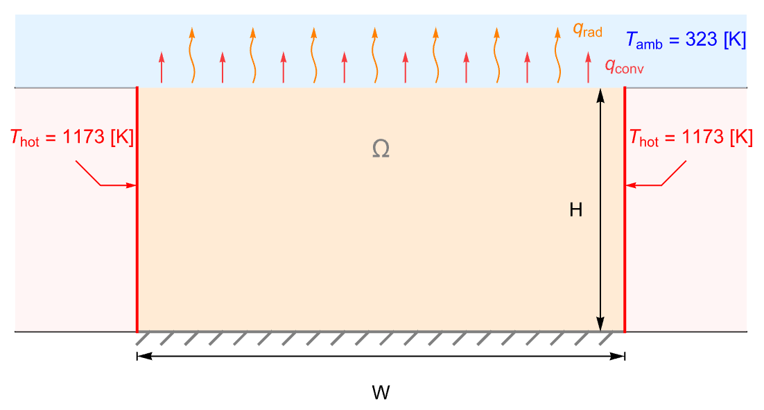
The following 2D stationary example [15] demonstrates a typical workflow of heat transfer modeling.
The model domain ![]() of width
of width ![]() and height of
and height of ![]() is a ceramic strip that is embedded in a high-thermal-conductive material. The side boundaries of the strip are maintained at a constant temperature
is a ceramic strip that is embedded in a high-thermal-conductive material. The side boundaries of the strip are maintained at a constant temperature ![]() . The top surface of the strip is losing heat via both thermal convection and thermal radiation to the ambient environment at
. The top surface of the strip is losing heat via both thermal convection and thermal radiation to the ambient environment at ![]() . The bottom boundary, however, is assumed to be thermally insulated.
. The bottom boundary, however, is assumed to be thermally insulated.
Our goal is to find the steady-state temperature distribution of the ceramic strip.
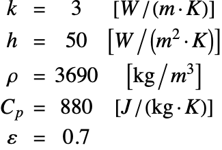
The thermal conductivity ![]() , heat transfer coefficient
, heat transfer coefficient ![]() , density
, density ![]() , heat capacity
, heat capacity ![]() and emissivity
and emissivity ![]() of the ceramic trip are given by:
of the ceramic trip are given by:
A default thermally insulated boundary condition is implicitly applied on the remaining bottom boundary.
In the steady-state, the minimum temperature is found on the top surface that is cooled by both convection and radiation. The defined temperature at the side is the maximum temperature since heat diffuses into the medium from the sides.
The setting of thermal boundary conditions will be explained in detail in a following section: Boundary Conditions in Heat Transfer.
Source Types
The source term ![]() in the heat equation (16) is used to model internal heat generation (
in the heat equation (16) is used to model internal heat generation (![]() ) or absorption (
) or absorption (![]() ) within the domain. Based on their shape heat sources are categorized as a Volumetric Heat Source, Layer Heat Source and Point Heat Source.
) within the domain. Based on their shape heat sources are categorized as a Volumetric Heat Source, Layer Heat Source and Point Heat Source.
It is important that the mesh conforms to the geometrical bounds of the source term ![]() , either by explicitly generating the mesh for them or by making use of the MeshRefinementFunction.
, either by explicitly generating the mesh for them or by making use of the MeshRefinementFunction.
A volumetric heat source ![]() can be used to model an arbitrarily shaped heat source (
can be used to model an arbitrarily shaped heat source (![]() ) or heat sink (
) or heat sink (![]() ) within the domain. The corresponding source strength
) within the domain. The corresponding source strength ![]() denotes the rate of an internal heating or cooling per unit volume.
denotes the rate of an internal heating or cooling per unit volume.
The term volumetric heat source may be a bit misleading. This is best seen by looking at the unit of a volumetric heat source ![]() that depends on the dimension of the system. In a 1D domain (
that depends on the dimension of the system. In a 1D domain (![]() ), 2D domain (
), 2D domain (![]() ) and in a 3D domain (
) and in a 3D domain (![]() )
) ![]() has a unit of
has a unit of ![]() ,
, ![]() and
and ![]() , respectively. So the name comes from the 3D incarnation of the heat source but is used in other dimensions as well.
, respectively. So the name comes from the 3D incarnation of the heat source but is used in other dimensions as well.
In the following 2D example a rectangular heat source ![]() is introduced to heat up the domain. The source strength is fixed at
is introduced to heat up the domain. The source strength is fixed at ![]() .
.
For more involved shapes of a heat source, the function RegionMember can be used to specify the source region ![]() .
.
In this case, however, because the shape of the heat source is simple we can simply specify the formula of the source region ![]() by making use of an If statement. This will lead to a more efficient time integration. The reason the If statement is more efficient is that it can be automatically compiled while the RegionMemberFunction can not be compiled.
by making use of an If statement. This will lead to a more efficient time integration. The reason the If statement is more efficient is that it can be automatically compiled while the RegionMemberFunction can not be compiled.
The most accurate and efficient method to deal with heat sources is by element makers as then the mesh will have a specific subregion for the heat source which will result in an accurate solution. More information on markers and their generation in meshes can be found in the Element Mesh Generation tutorial.
An example that uses element makers for the heat source set up is presented in the appendix section: Modeling Heat Source by Element Markers.
See this note about improving the visual quality of the animation.
The simulation begins with an undisturbed domain where ![]() . With a volumetric heat source
. With a volumetric heat source ![]() placed in the domain, thermal energy is generated and gradually heats up the domain. The speed of the heat transfer depends on the heat conductivity
placed in the domain, thermal energy is generated and gradually heats up the domain. The speed of the heat transfer depends on the heat conductivity ![]() and the heat capacity
and the heat capacity ![]() of the material.
of the material.
A layer heat source models a heat source (![]() ) or heat sink (
) or heat sink (![]() ) that is too thin to have a thickness in the model geometry. A layer heat source can be made use of in 3D and in 2D domains. In 1D domains a layer heat is the same dimension as the simulation domain, which is not possible. The corresponding source strength
) that is too thin to have a thickness in the model geometry. A layer heat source can be made use of in 3D and in 2D domains. In 1D domains a layer heat is the same dimension as the simulation domain, which is not possible. The corresponding source strength ![]() denotes the rate of the internal heating or cooling per unit area.
denotes the rate of the internal heating or cooling per unit area.
Here ![]() is a Dirac delta function at the source location
is a Dirac delta function at the source location ![]() .
.
The Dirac delta function, however, poses a problem in numerical simulations as it can not be resolved in the discretized spatial domain. This is because the Dirac delta function is singular at the source location ![]() . Hence, an approximation to the Dirac delta function is needed. The process of approximating the Dirac delta function is called regularization.
. Hence, an approximation to the Dirac delta function is needed. The process of approximating the Dirac delta function is called regularization.
There are various regularized delta functions ![]() available [17][18]. In this tutorial we choose:
available [17][18]. In this tutorial we choose:
where ![]() is the regularization parameter that controls the support of the regularized delta functions
is the regularization parameter that controls the support of the regularized delta functions ![]() . Typically
. Typically ![]() should have a size comparable to the mesh spacing
should have a size comparable to the mesh spacing ![]() .
.
The units of a layer heat source ![]() depend on the dimension of the system, much like the volumetric heat source. In a 3D domain (
depend on the dimension of the system, much like the volumetric heat source. In a 3D domain (![]() ) the layered heat source
) the layered heat source ![]() is presented as a 2D surface, and thus has a unit of
is presented as a 2D surface, and thus has a unit of ![]() . In 2D domain (
. In 2D domain (![]() ), however, the geometry of a layer heat source renders into a 1D line, and the unit of
), however, the geometry of a layer heat source renders into a 1D line, and the unit of ![]() becomes
becomes ![]() . In 1D there is no layer heat source. In that case a point heat source should be used instead.
. In 1D there is no layer heat source. In that case a point heat source should be used instead.
In the following 2D example a layer heat source ![]() is added at
is added at ![]() to heat up the domain. The source strength is fixed at
to heat up the domain. The source strength is fixed at ![]() .
.
To accommodate the layered heat source ![]() in the mesh, a boundary mesh with the line at
in the mesh, a boundary mesh with the line at ![]() is generated.
is generated.
More information on the mesh generation can be found in the Element Mesh Generation tutorial.
To utilize the regularized delta function ![]() , we choose the regularization parameter to be half of the mesh spacing:
, we choose the regularization parameter to be half of the mesh spacing: ![]() .
.
See this note about improving the visual quality of the animation.
The simulation begins with an undisturbed domain where ![]() . With a layer heat source
. With a layer heat source ![]() placed at
placed at ![]() , the thermal energy is generated and propagates towards both sides of the domain. The speed of the heat transfer depends on the heat conductivity
, the thermal energy is generated and propagates towards both sides of the domain. The speed of the heat transfer depends on the heat conductivity ![]() and the heat capacity
and the heat capacity ![]() of the material.
of the material.
Note that a layered heat source is not limited to a linear surface (![]() ) or a straight line (
) or a straight line (![]() ). The following 2D example demonstrates a layer heat source
). The following 2D example demonstrates a layer heat source ![]() with a curved source region.
with a curved source region.
More information on the mesh generation can be found in the Element Mesh Generation tutorial.
See this note about improving the visual quality of the animation.
With a curved layered heat source ![]() heading downward, most of the heat is transported toward the lower half
heading downward, most of the heat is transported toward the lower half ![]() of the domain.
of the domain.
A point heat source ![]() can be used to model an internal heat source (
can be used to model an internal heat source (![]() ) or heat sink (
) or heat sink (![]() ) that is considered to have no spatial extension. A point heat source can be made use of in 3D and in 2D domains. In 1D domains a point heat is corresponds to a boundary condition. The corresponding source strength
) that is considered to have no spatial extension. A point heat source can be made use of in 3D and in 2D domains. In 1D domains a point heat is corresponds to a boundary condition. The corresponding source strength ![]() denotes the rate of the internal heating or cooling at the source point
denotes the rate of the internal heating or cooling at the source point ![]() in unit power.
in unit power.
Since the point heat source has no spatial extension in all directions, the Dirac delta function ![]() should be applied on each dimension (i.e.
should be applied on each dimension (i.e. ![]() ) of the modeling domain
) of the modeling domain ![]() :
:
In the following 2D example a point heat source ![]() is added at
is added at ![]() to heat up the domain. The source strength
to heat up the domain. The source strength ![]() is fixed at
is fixed at ![]() .
.
See this note about improving the visual quality of the animation.
The simulation begins with an undisturbed domain where ![]() . With a point heat source
. With a point heat source ![]() placed in the domain, thermal energy is generated and spreads out in all directions. The speed of the heat transfer depends on the heat conductivity
placed in the domain, thermal energy is generated and spreads out in all directions. The speed of the heat transfer depends on the heat conductivity ![]() and the heat capacity
and the heat capacity ![]() of the material.
of the material.
Anisotropic and Orthotropic Heat Transfer
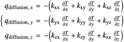
In the previous sections we assumed that heated medium is isotropic, that is, the rate of heat transfer is independent of its direction given the same the temperature gradient ![]() . In reality, however, a medium may be anisotropic. This means that heat diffuses in different directions with a different rate. The diffusion term (19) is then rewritten as:
. In reality, however, a medium may be anisotropic. This means that heat diffuses in different directions with a different rate. The diffusion term (19) is then rewritten as:
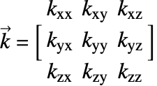
where ![]() is the thermal conductivity tensor.
is the thermal conductivity tensor. ![]() and
and ![]() are called the principal conductivity coefficients and off-diagonal conductivity coefficients, respectively.
are called the principal conductivity coefficients and off-diagonal conductivity coefficients, respectively.
Based on Onsager's [20] principle of the thermodynamics of irreversible processes, the off-diagonal conductivity must obey the reciprocity relation [21]:
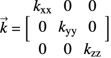
Orthotropic heat transfer is a special case of anisotropic heat transfer. Here the thermal conductivity of a material is symmetric along the principal directions ![]() ,
, ![]() and
and ![]() and the off-diagonal conductivity coefficients are zero. This behaviour can be seen, for example, in fiber composite materials. Then the thermal conductivity tensor becomes:
and the off-diagonal conductivity coefficients are zero. This behaviour can be seen, for example, in fiber composite materials. Then the thermal conductivity tensor becomes:
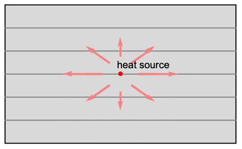
As an example, consider a 2D composite material with layered-like structure:
This case is the orthotropic case where the heat transfer is more efficient horizontally. Should the thermal conductivity tensor be described by:
See this note about improving the visual quality of the animation.
Unlike the example shown in the previous section, in the case the heat transfer is faster in the horizontal direction, resulting in a higher temperature zone within ![]() .
.
Nonlinear Heat Transfer
In the previous sections we assumed that the PDE coefficients namely, the density ![]() , the heat capacity
, the heat capacity ![]() and the thermal conductivity
and the thermal conductivity ![]() are independent of the temperature field
are independent of the temperature field ![]() . In reality, however, these parameters might change significantly with temperature, especially for pure metals.
. In reality, however, these parameters might change significantly with temperature, especially for pure metals.
As an example, consider a 1D heat transfer model with an initial temperature field at ![]() and a temperature-dependent thermal conductivity
and a temperature-dependent thermal conductivity ![]() :
:
Equation (22) is a nonlinear heat transfer model since the conductivity coefficient ![]() in the PDE model now depends on the temperature
in the PDE model now depends on the temperature ![]() itself.
itself.
To heat up the domain, a constant heat flux ![]() is applied on the left hand boundary.
is applied on the left hand boundary.
To understand the effects of the nonlinearity compare to a linear heat transfer PDE.
The simulation begins with an undisturbed domain where ![]() . With a constant heat flux
. With a constant heat flux ![]() applied on the left side, thermal energy is then transferred across the boundary and heats up the domain.
applied on the left side, thermal energy is then transferred across the boundary and heats up the domain.
For the non-linear model, as the temperature ![]() increases the thermal conductivity
increases the thermal conductivity ![]() will increase correspondingly, which further speeds up the heat transfer and results in a flatter temperature field.
will increase correspondingly, which further speeds up the heat transfer and results in a flatter temperature field.
Heat Transfer with Events
A common topic in heat transfer modeling is to simulate dynamic or pulsed thermal loads. That is, a heat flux that turns on and off under different conditions. In such cases we can make use of WhenEvent to construct and efficiently solve the heat transfer model.
Consider a 1D room model where heat continuously flows out of the room at both sides. A heater is placed in the domain to warm up the room, but will only turn on when the temperature at the center ![]() drops below the threshold temperature
drops below the threshold temperature ![]() . To prevent overheating the heater will turn off when
. To prevent overheating the heater will turn off when ![]() is above
is above ![]() .
.
To model the conditional heating of the heater, we apply a volumetric heat source ![]() using WhenEvent. The heat source
using WhenEvent. The heat source ![]() is switched on and off when the central temperature
is switched on and off when the central temperature ![]() reaches
reaches ![]() or
or ![]() .
.
To model the cooling of the room, a constant cooling flux ![]() is applied on both ends of the domain.
is applied on both ends of the domain.
Next, we define the heat transfer PDE with the conditional heat source ![]() . Since the heater is off at the beginning, the initial value of the heat source is set at
. Since the heater is off at the beginning, the initial value of the heat source is set at ![]() .
.
To solve this heat transfer PDE we specify ![]() as a discrete variable, which means it only changes at discrete times during the temporal integration by NDSolve.
as a discrete variable, which means it only changes at discrete times during the temporal integration by NDSolve.
The simulation begins with an uniform temperature at ![]() . With a constant cooling flux
. With a constant cooling flux ![]() applied on both sides, heat continuously flows out of the domain and brings down the room temperature. The heat source
applied on both sides, heat continuously flows out of the domain and brings down the room temperature. The heat source ![]() is then turned on and off when the central temperature
is then turned on and off when the central temperature ![]() reaches
reaches ![]() or
or ![]() , resulting in an oscillating temperature field.
, resulting in an oscillating temperature field.
While it would also be possible to make use of an If statement to model the dynamic or pulsed heat source, the use of WhenEvent has the distinct advantage that NDSolve has special mechanisms build in to detect the events during the time integration. This mechanism may not be available when modeling the pulsed heat source with an If or similar statement.
Details about modeling heat pulses are presented in the appendix section: Possible Issues and Workarounds for Modeling Heat Pulses.
Heat Transfer in Porous Media
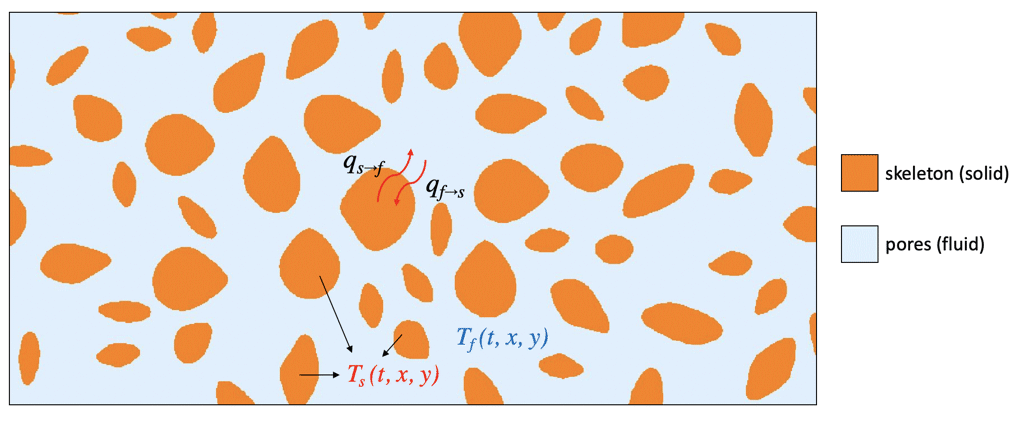
Porous media are multiphase objects with a solid skeleton portion and a porous region that is filled with a fluid. Due to its special thermal and mechanical properties, porous materials have been widely used in many industrial applications such as vibration suppression, heat insulation and sound absorption.
To model heat transfer within a porous medium, one approach, called a direct approach, is to build a coupled PDE with two heat equations with material coefficients suitable for each phase. One equation describes the temperature field ![]() in the solid region and the other equation models the temperature
in the solid region and the other equation models the temperature ![]() in the fluid region:
in the fluid region:
Here the subscript ![]() denotes the parameters for the solid phase and
denotes the parameters for the solid phase and ![]() for the fluid phase. The two equations are coupled by the volume fraction
for the fluid phase. The two equations are coupled by the volume fraction ![]() of each phase, and the heat exchange between two phases are accounted for explicitly by an additional heat source/sink term
of each phase, and the heat exchange between two phases are accounted for explicitly by an additional heat source/sink term ![]() on the right hand side.
on the right hand side.
However, to make use of this approach it is required to reproduce the entire pore structure of the domain. Due to the geometric complexify of the microscopic porous structure, a fine finite element mesh may be required to resolve the geometry accurately and thus a significant computational cost to solve the model can be expected.
An alternate approach is to model pores on a macroscopic scale. In this case the heat transfer model uses an average temperature field to describe the entire porous structure of both phases. To do so volume-averaged effective thermal properties are used, and the model can be expressed by a single heat equation:
Here ![]() is the effective volumetric heat capacity and
is the effective volumetric heat capacity and ![]() is the effective heat conductivity, which are computed based on the volume fraction
is the effective heat conductivity, which are computed based on the volume fraction ![]() and the properties of each phase.
and the properties of each phase.
Assuming a porous medium to be fully saturated, the volume fraction of both phases can be related by: ![]() . Then the equation (23) becomes:
. Then the equation (23) becomes:
Note that the fluid's volume fraction ![]() is also known as the porosity of the medium. For the sake of simplicity we will omit its subscript
is also known as the porosity of the medium. For the sake of simplicity we will omit its subscript ![]() in the following section.
in the following section.
As an example, consider a 2D heat transfer model of a porous medium. A fluid flow is passing through the domain ![]() with a width of
with a width of ![]() and a height of
and a height of ![]() , and a constant heat flux is applied on the left surface to heat up a domain. To understand the effects of the porosity on the heat transfer, the model will be solved with three different porosity values of
, and a constant heat flux is applied on the left surface to heat up a domain. To understand the effects of the porosity on the heat transfer, the model will be solved with three different porosity values of ![]() ,
, ![]() and
and ![]() (purely fluidic medium).
(purely fluidic medium).
Equation (24) has an effective volumetric heat capacity in front of the time derivative and at the same time uses material parameters for the fluidic phase. To accommodate for that the equation is in part generated with HeatTransferPDEComponent and an additional time derivative term. For that the model variables include a time dependent variable but not the time variable itself. The time derivative with it's effective volumetric heat capacity will be added manually.
To heat up the domain, a constant heat flux ![]() into the domain is applied on the left surface at
into the domain is applied on the left surface at ![]() .
.
Note that the temperature field is symmetric in the ![]() direction.
direction.
To study the effects of the porosity on the heat transfer, we can compare the temperature evolution along the ![]() axis at three different porosity values of
axis at three different porosity values of ![]() ,
, ![]() and
and ![]() (purely fluidic medium).
(purely fluidic medium).
Since the heat capacity value in the solid phase is smaller than in the fluid phase: ![]() , the medium with a larger amount of solid (i.e. lower porosity
, the medium with a larger amount of solid (i.e. lower porosity ![]() ) will be more susceptible to the temperature change. This can be verified by computing the effective volumetric heat capacity
) will be more susceptible to the temperature change. This can be verified by computing the effective volumetric heat capacity ![]() at
at ![]() ,
, ![]() and
and ![]() .
.
Note that for ![]() the effective heat capacity
the effective heat capacity ![]() is the smallest.
is the smallest.
Heat Transfer Model with Mixed Dimensions
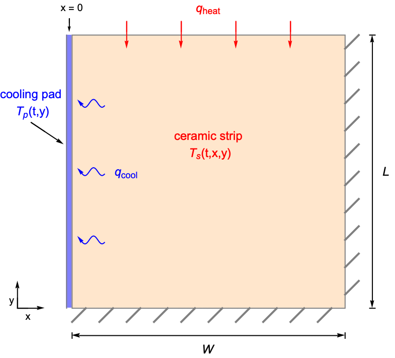
The following section demonstrates how to model heat transfer phenomena defined in different spatial dimensions. As an example, consider a 2D ceramic strip with an uniform initial temperature at ![]() . At the left surface the ceramic is cooled down by attaching to a thin pad with a cooling flux through it. The cooling flux
. At the left surface the ceramic is cooled down by attaching to a thin pad with a cooling flux through it. The cooling flux ![]() is proportional to the temperature difference between the pad and the ceramic with a heat transfer coefficient
is proportional to the temperature difference between the pad and the ceramic with a heat transfer coefficient ![]() .
.
A constant heat flux ![]() is applied on the top of the ceramic. The right and bottom surfaces of the ceramic are assumed to be thermally insulated.
is applied on the top of the ceramic. The right and bottom surfaces of the ceramic are assumed to be thermally insulated.
To solve for the temperature field ![]() of the ceramic, a first idea might be to build a single 2D system and model the cooling pad as a heat flux boundary condition. In this example, however, the cooling flux
of the ceramic, a first idea might be to build a single 2D system and model the cooling pad as a heat flux boundary condition. In this example, however, the cooling flux ![]() depends not only on
depends not only on ![]() but also on the pad temperature
but also on the pad temperature ![]() . In order to determine the value of the pad temperature
. In order to determine the value of the pad temperature ![]() it is necessary to also model the heat transfer in the thin cooling pad.
it is necessary to also model the heat transfer in the thin cooling pad.
Assuming that the cooling pad to be much thinner than the width of the ceramic, the temperature variation of the pad in the ![]() direction can be neglected. The cooling pad can thus be modeled as a 1D region while the ceramic strip is modeled as a 2D region. In other words a mixed dimensional model can be used.
direction can be neglected. The cooling pad can thus be modeled as a 1D region while the ceramic strip is modeled as a 2D region. In other words a mixed dimensional model can be used.
For simplicity the heat transfer coefficient ![]() and the thermal conductivity
and the thermal conductivity ![]() , density
, density ![]() and heat capacity
and heat capacity ![]() for both the ceramic strip and the pad are set to one.
for both the ceramic strip and the pad are set to one.
The temperature field ![]() within the ceramic strip is described by a 2D heat equation:
within the ceramic strip is described by a 2D heat equation:
The pad is described by the 1D domain along the ![]() axis
axis ![]() , which coincides with the left surface of the ceramic strip. A 1D heat equation can be used to model the pad temperature
, which coincides with the left surface of the ceramic strip. A 1D heat equation can be used to model the pad temperature ![]() along the 1D pad region as:
along the 1D pad region as:
However, to solve a coupled PDE system, NDSolve requires all the dependent variables to have the same spatial dimensionality. For this reason alone we have to introduce a "fictitious dimension" for the pad temperature ![]() in the
in the ![]() direction, yielding:
direction, yielding:
That is, we will be solving the pad temperature ![]() not only in the 1D pad region, but also the entire 2D domain of the ceramic strip. However, since
not only in the 1D pad region, but also the entire 2D domain of the ceramic strip. However, since ![]() is just a fictitious dimension for the pad there is no physical meaning to a
is just a fictitious dimension for the pad there is no physical meaning to a ![]() value within the ceramic region
value within the ceramic region ![]() , which means the resulting pad temperature field
, which means the resulting pad temperature field ![]() will only be valid along the 1D pad region on the
will only be valid along the 1D pad region on the ![]() axis
axis ![]() .
.
Next we need to consider the heat exchange between the cooling pad and the ceramic strip. From the perspective of the ceramic, heat is lost through the left ceramic boundary to the pad, and can be modeled with a heat flux boundary condition.
From the perspective of the cooling pad, heat is gained from the ceramic strip over the entire pad domain. This can be modeled by a heat source term ![]() in the equation (25).
in the equation (25).
Due to the law of energy balance, the heat source ![]() of the pad should have the same magnitude but an opposite sign from the cooling flux
of the pad should have the same magnitude but an opposite sign from the cooling flux ![]() of the ceramic.
of the ceramic.
A constant heating flux ![]() is applied on the upper surface of the ceramic.
is applied on the upper surface of the ceramic.
See this note about improving the visual quality of the animation.
Next we inspect the pad temperature ![]() within the 1D pad region
within the 1D pad region ![]() , and compare it to the ceramic temperature
, and compare it to the ceramic temperature ![]() on the left ceramic surface. A custom function, TwoAxisPlot, is defined and applied to rescale the temperature range in the plot for better visualization.
on the left ceramic surface. A custom function, TwoAxisPlot, is defined and applied to rescale the temperature range in the plot for better visualization.
Since the heat gain of the pad depends on the ceramic temperature ![]() , the pad temperature
, the pad temperature ![]() follows a similar pattern with
follows a similar pattern with ![]() along the left ceramic surface
along the left ceramic surface ![]() .
.
Introducing a fictitious dimension in the coupled PDE system enables solving a mixed dimensional model involving a 1D and a 2D heat equation. This technique is known as the "Fictitious Domain Method", and can also be applied to other dimensions (1, 2 or 3D) in a similar manner.
Heat Transfer with Phase Change
A phase change in thermodynamics denotes the phenomenon where materials transit from one state (solid, liquid, gas, plasma) to another, which only occurs at certain temperature and pressure and when sufficient energy is added or removed from the system. The energy associated with the phase change, which is known as the latent heat ![]() , is used to alters the molecular structure instead of creating a temperature change of the material.
, is used to alters the molecular structure instead of creating a temperature change of the material.
As an example, consider the following 1D model that describes the ice-to-water phase change along a ![]() rod of ice. The rod has an initial temperature of
rod of ice. The rod has an initial temperature of ![]() , and a constant heat flux
, and a constant heat flux ![]() is applied at the left end to melt the rod. At the right end the rod is assumed to be thermally insulated.
is applied at the left end to melt the rod. At the right end the rod is assumed to be thermally insulated.
In the heat transfer model, instead of simulating the phase transition exactly at the phase change temperature ![]() , we assume that the transition occurs in a temperature interval:
, we assume that the transition occurs in a temperature interval: ![]() to
to ![]() . The material phase during the transition is then described by a smoothed step function
. The material phase during the transition is then described by a smoothed step function ![]() , which denotes the ratio of the original phase to the new phase within the material.
, which denotes the ratio of the original phase to the new phase within the material.
Within the temperature interval: ![]() , the equivalent density
, the equivalent density ![]() and conductivity
and conductivity ![]() are given by:
are given by:
The equivalent specific heat capacity ![]() , however, should include an extra term
, however, should include an extra term ![]() to account for the latent heat
to account for the latent heat ![]() required for the phase transition. Here
required for the phase transition. Here ![]() denotes the distribution of the latent heat
denotes the distribution of the latent heat ![]() during the phase change, and is approximated by a regularized delta function around the phase change temperature
during the phase change, and is approximated by a regularized delta function around the phase change temperature ![]() :
:
Note that the integral of ![]() equals to the latent heat
equals to the latent heat ![]() required for the phase change:
required for the phase change:
The equivalent heat capacity ![]() is then given by:
is then given by:
A default thermally insulated boundary condition is implicitly applied at the right end of the rod.
To better understand the effects of the latent heat ![]() on the phase change, we will compare the above result with a solution that neglects the latent heat.
on the phase change, we will compare the above result with a solution that neglects the latent heat.
Heat Transfer with Model Order Reduction
Some times one want to re-run the same heat transfer simulation with different initial data. In this case model order reduction can be of help. The idea behind model order reduction is make use of the discretization of the PDE and find a similar discretization that can be time integrated much more efficiently. In order to perform a model order reduction access to the discretization NDSolve makes is necessary. This is currently not possible on the NDSolve level but requires a bit of programing and is explained in the section Model Order Reduction of Transient PDEs with Stationary Coefficients and Stationary Boundary Conditions in the Finite Element Programming tutorial.
Boundary Conditions in Heat Transfer
The most common boundary conditions in heat transfer modeling can be modeled with DirichletCondition, NeumannValue and PeriodicBoundaryCondition, and can be categorized in the following four types:
- Dirichlet type boundary conditions. This type of boundary condition specifies the temperature
 at the boundary, and can be modeled with DirichletCondition.
- Neumann type boundary conditions. This type of boundary condition specifies the heat flux
 at the boundary, and can be modeled with NeumannValue.
- Robin type boundary conditions. This type of boundary condition specifies the relation between the temperature
 and its normal derivatives at the boundary, and can modeled with a NeumannValue since Robin type boundary conditions are technically generalized Neumann boundary conditions.
- Periodic boundary conditions. This type of boundary condition specifies the temperature
 at one part of the boundary to be the same at another part, and can be modeled with PeriodicBoundaryCondition.
Under these four types, the following boundary conditions are introduced:
The following section describes several physical boundaries common in heat transfer and how they can be modeled with the use of DirichletCondition, NeumannValue and PeriodicBoundaryCondition. For this purpose the boundary condition currently discussed is always on the left hand side of the simulation domain. In some examples additional boundary conditions are on the right hand side to better demonstrate the behaviour of the boundary condition on the left hand side.
Temperature Surface Boundary Condition
The purpose of a temperature surface boundary condition is to set a specific temperature on some part of the boundary.
With a specified temperature ![]() on the boundary
on the boundary ![]() , the temperature surface condition is given by:
, the temperature surface condition is given by:
We speak of a temperature boundary condition when the surface temperature ![]() is prescribed on a boundary. The surface temperature
is prescribed on a boundary. The surface temperature ![]() can either be a constant or time-dependent value, and is set with a DirichletCondition in the heat transfer PDE model.
can either be a constant or time-dependent value, and is set with a DirichletCondition in the heat transfer PDE model.
To model, for example, a heating wall that sends thermal energy into the domain, a transient surface temperature ![]() can be set up at the left end. Note that a Neumann zero condition is implicitly applied at the right end as a thermal insulated boundary.
can be set up at the left end. Note that a Neumann zero condition is implicitly applied at the right end as a thermal insulated boundary.
Here a smoothed step function is used to described the profile of the surface temperature ![]() from
from ![]() to
to ![]() . The parameters
. The parameters ![]() and
and ![]() are arbitrarily chosen to simulate the heating process.
are arbitrarily chosen to simulate the heating process.
The simulation begins with an undisturbed domain where ![]() . As the surface temperature
. As the surface temperature ![]() increases at the left boundary, the excess thermal energy is then passed to the right and brings up the the temperature throughout the domain. The speed of the heat transfer depends on the heat conductivity
increases at the left boundary, the excess thermal energy is then passed to the right and brings up the the temperature throughout the domain. The speed of the heat transfer depends on the heat conductivity ![]() and the heat capacity
and the heat capacity ![]() of the material.
of the material.
Heat Flux Boundary Condition
The purpose of a heat flux boundary condition is to model the amount of thermal energy flowing into or out of some part of the boundary.
With a prescribed heat flux ![]() on the boundary
on the boundary ![]() , the heat flux boundary condition is given by:
, the heat flux boundary condition is given by:
A boundary where the heat flux ![]() normal to the boundary is specified and not equal to zero is called a heat flux boundary:
normal to the boundary is specified and not equal to zero is called a heat flux boundary:
By convention a negative sign is added in front of ![]() to indicates that the heat flux is specified opposite to the outward normal
to indicates that the heat flux is specified opposite to the outward normal ![]() . Therefore, a positive value of
. Therefore, a positive value of ![]() denotes the inward heat flux where the thermal energy enters the domain, and a negative
denotes the inward heat flux where the thermal energy enters the domain, and a negative ![]() denotes an outward flux.
denotes an outward flux.
Fourier's law of thermal conduction (26) relates the heat flux ![]() with the temperature gradient
with the temperature gradient ![]() :
:
Inserting (27) into (28), the heat flux boundary condition can be written as:
Note that the unit of a heat flux ![]() depends on the dimension of the boundary. In 1D (
depends on the dimension of the boundary. In 1D (![]() ), 2D (
), 2D (![]() ) and 3D domain (
) and 3D domain (![]() ),
), ![]() has a unit of
has a unit of ![]() ,
, ![]() and
and ![]() , respectively.
, respectively.
In the following example a transient heat flux ![]() is applied on the left boundary when
is applied on the left boundary when ![]() to heat up the domain.
to heat up the domain.
The profile of the heat flux is defined as:
With the heat flux ![]() applied on the left boundary, thermal energy flows across the boundary and gradually heats up the domain. The heat flux is turned off at time
applied on the left boundary, thermal energy flows across the boundary and gradually heats up the domain. The heat flux is turned off at time ![]() . The uneven temperature field is then smoothed out over time by the internal heat transfer.
. The uneven temperature field is then smoothed out over time by the internal heat transfer.
Note that the value of the heat flux is related to the temperature gradient ![]() by Fourier's law:
by Fourier's law: ![]() . That is, the heat flux
. That is, the heat flux ![]() directly controls the temperature gradient normal to the boundary.
directly controls the temperature gradient normal to the boundary.
Thermally Insulated Boundary Condition
The purpose of a thermally insulated boundary condition is to model a boundary where there is no heat flux across it.
A thermally insulated boundary condition is given by:
If on some part of the boundary no boundary condition is set an implicit Neumann zero boundary condition is used.
A thermally insulated condition denotes a boundary where there is no heat flux across it:
Inserting (29) into the heat flux boundary condition (30), then the thermally insulated boundary condition can be written as:
In the following example an insulated boundary is placed on the left hand boundary, and a constant heat flux ![]() is added on the right end to serve as a heat source.
is added on the right end to serve as a heat source.
If no boundary condition is specified on any part of the boundary then by default a Neumann zero boundary condition is implicitly used. This implies that the thermally insulated boundary is the default boundary condition used if no boundary condition is specified at a given boundary.
With a constant heat flux enforced on the right boundary, the temperature gradually increases within the domain. On the insulated boundary at the left end, however, the temperature gradient ![]() remains at zero at all times.
remains at zero at all times.
Since the temperature gradient ![]() is related to the heat flux
is related to the heat flux ![]() by Fourier's law:
by Fourier's law: ![]() , a zero temperature gradient implies a zero heat flux on the boundary (i.e. thermal insulated boundary).
, a zero temperature gradient implies a zero heat flux on the boundary (i.e. thermal insulated boundary).
Symmetry Boundary Condition
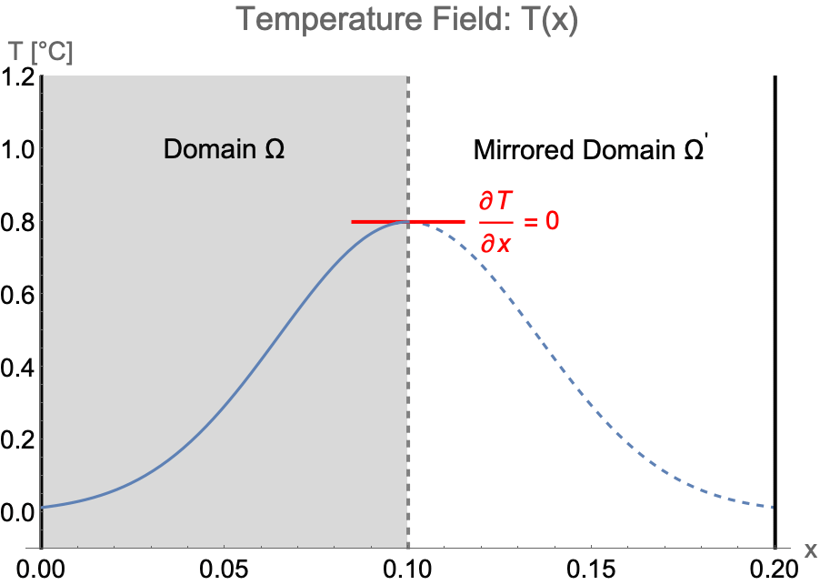
A symmetry boundary condition is used when the computational domain, and the expected temperature field, have mirror symmetry along an axis of the simulation domain.
The symmetry boundary condition is given by:
If on some part of the boundary no boundary condition is set an implicit Neumann zero boundary condition is used.
A symmetry boundary condition is used to reduce the extent of the computational domain to a symmetric sub-domain of the full physical model geometry. This allows for a faster solution process with a lower memory requirement.
Consider the case of solving the temperature field of a 1D system from ![]() to
to ![]() . If the temperature pattern is expected to have a mirror symmetry along
. If the temperature pattern is expected to have a mirror symmetry along ![]() , we can efficiently construct the simulation domain
, we can efficiently construct the simulation domain ![]() with only the left half of the system. Then a symmetry boundary condition should be applied at
with only the left half of the system. Then a symmetry boundary condition should be applied at ![]() .
.
Due to the symmetry, the temperature gradient at the symmetry boundary will remain at zero at all time, which implies a zero heat flux across the boundary. Therefore, a symmetry boundary condition is equivalent to a thermally insulated boundary condition.
Outflow Boundary Condition
If the heat transfer occurs in a fluid medium where the flow velocity ![]() , then an outflow boundary condition is used to model an outlet where heat is transferred out of the domain by fluid flow.
, then an outflow boundary condition is used to model an outlet where heat is transferred out of the domain by fluid flow.
When modeling heat transfer in a fluid medium, the outflow boundary condition at the outlet ![]() is given by:
is given by:
If on some part of the boundary no boundary condition is set an implicit Neumann zero boundary condition is used.
When modeling heat transfer with a fluid flow, the diffusion heat flux ![]() is set to zero at the flow outlet boundary. This condition means that the temperature field of the flow outside the domain is assumed to have no impact on the flow inside the modeling domain
is set to zero at the flow outlet boundary. This condition means that the temperature field of the flow outside the domain is assumed to have no impact on the flow inside the modeling domain ![]() .
.
The outflow boundary condition can only be applied on fully-developed flows. That is, at the flow outlet the velocity profile ![]() is unchanging in the flow direction.
is unchanging in the flow direction.
In a case where there is recirculation through the outlet boundary, which often happens for turbulent flow, the reentering flow will affect the temperature field of the flow inside the domain and break the zero diffusion flux assumption. In this situation the outflow boundary condition is no longer applicable.
Since the outflow boundary condition is essentially a Neumann zero condition, it will be implicitly applied if no boundary condition is specified at a given boundary.
Convective Boundary Condition
The purpose of a convective boundary condition is to model thermal energy transferred across a boundary induced by a flow adjacent to the same part of the boundary.
Given the profile of an external temperature ![]() and a heat transfer coefficient
and a heat transfer coefficient ![]() on the boundary
on the boundary ![]() , the convective boundary condition is given by:
, the convective boundary condition is given by:
With the existence of a fluid flowing adjacent to the boundary surface, part of the thermal energy will be transferred across the boundary through the movement of fluid particles, which is known as convective heating or cooling.
In 1701, Newton found that the rate of convective heat transfer between two media is proportional to their temperature difference. The convective heat flux is therefore defined as:
Here ![]() denotes the temperature of the external fluid, and
denotes the temperature of the external fluid, and ![]() in units of
in units of ![]() is the convective heat transfer coefficient. The heat transfer coefficient is determined experimentally and depends on material properties like density
is the convective heat transfer coefficient. The heat transfer coefficient is determined experimentally and depends on material properties like density ![]() , the thermal diffusivity
, the thermal diffusivity ![]() and the flow situation of the external fluid such as viscosity
and the flow situation of the external fluid such as viscosity ![]() and Rayleigh number
and Rayleigh number ![]() .
.
The approximate range of the convection heat transfer coefficients ![]() are presented in following table:
are presented in following table:
Several empirical based formulas are also built [31,32] to estimate the heat transfer coefficient ![]() in different situations.
in different situations.
Inserting (33) into the heat flux boundary condition (34), the convective boundary condition can be written as:
In the following example a constant external flow at ![]() is applied on the left boundary to heat up the domain
is applied on the left boundary to heat up the domain ![]() of an initial temperature field at
of an initial temperature field at ![]() . The convection heat transfer through the boundary is modeled by the convective boundary condition with a given heat transfer coefficient
. The convection heat transfer through the boundary is modeled by the convective boundary condition with a given heat transfer coefficient ![]() .
.
With the external flow flowing left of the left boundary, excess thermal energy is transferred across the boundary into the domain. Since the convective heat flux is proportional to the temperature difference across the boundary: ![]() , the temperature gradient
, the temperature gradient ![]() at the left boundary will gradually decrease as the temperature
at the left boundary will gradually decrease as the temperature ![]() at the boundary approaches the external temperature
at the boundary approaches the external temperature ![]() .
.
Thermal Radiation Boundary Condition
The purpose of a thermal radiation boundary condition is to model heating or cooling through radiation on some part of the boundary.
Given an ambient temperature ![]() , the surface emissivity
, the surface emissivity ![]() and the Stefan-Boltzmann constant
and the Stefan-Boltzmann constant ![]() on the boundary
on the boundary ![]() , the thermal radiation boundary condition can be written as:
, the thermal radiation boundary condition can be written as:
All bodies with a temperature above the absolute zero (i.e. ![]() ) will constantly emit thermal energy through electromagnetic radiation. The amount of radiation depends on both body temperature and surface condition. For a perfect thermal radiator, a black body, the Stefan-Boltzmann law states that the emitting heat flux is proportional to the fourth power of the body's absolute temperature:
) will constantly emit thermal energy through electromagnetic radiation. The amount of radiation depends on both body temperature and surface condition. For a perfect thermal radiator, a black body, the Stefan-Boltzmann law states that the emitting heat flux is proportional to the fourth power of the body's absolute temperature:
where ![]() is the Stefan-Boltzmann constant.
is the Stefan-Boltzmann constant.
In practice, however, the actually emitted heat flux is less than that of the black body radiation by a fraction ![]() known as the "surface emissivity". The value of the emissivity is
known as the "surface emissivity". The value of the emissivity is ![]() and depends on factors such as physical properties and surface condition of the radiative body.
and depends on factors such as physical properties and surface condition of the radiative body.
The Stefan-Boltzmann law can be rewritten as:
Based on (35) we can formulate a radiation boundary condition by inspecting the net radiative heat flux ![]() across a boundary:
across a boundary:
The emitted, outgoing radiative flux ![]() from a boundary depends on its surface temperature
from a boundary depends on its surface temperature ![]() and the emissivity
and the emissivity ![]() by:
by:
At the same time, a boundary will absorb the radiation coming from the environment. This absorbed, incoming radiative flux ![]() is given by:
is given by:
Here ![]() is the ambient temperature and
is the ambient temperature and ![]() is the emissivity of the environment. Note that an extra term
is the emissivity of the environment. Note that an extra term ![]() , the surface absorptivity factor, is multiplied on the right hand side to account for the absorptivity of the boundary. This term denotes the ratio of the actual absorbed radiative flux to the total arriving flux.
, the surface absorptivity factor, is multiplied on the right hand side to account for the absorptivity of the boundary. This term denotes the ratio of the actual absorbed radiative flux to the total arriving flux.
Therefore, the net radiative heat flux across the boundary is given by:
To satisfy the thermodynamic equilibrium, for an arbitrary body the absorptivity ![]() should be equal to its emissivity
should be equal to its emissivity ![]() . This is known as the Kirchhoff's law of thermal radiation [36].
. This is known as the Kirchhoff's law of thermal radiation [36].
The equation (37) is then simplified to:
Assuming that the ambient surrounding behaves as a black body with the emissivity ![]() , the equation can be further simplified as:
, the equation can be further simplified as:
Inserting (38) into the heat flux boundary condition (39), then the radiative boundary condition is given by:
Note that the above derivation is performed based on the absolute temperature. That means the temperature terms in (40) have the unit of Kelvin ![]() .
.
To apply a radiation boundary condition in Celsius ![]() , an unit conversion should be done in (41) :
, an unit conversion should be done in (41) :
Here ![]() denotes the temperature of absolute zero.
denotes the temperature of absolute zero.
As an example consider the ambient temperature of ![]() and a surface emissivity
and a surface emissivity ![]() at the left hand boundary. The net radiative heat flux across the boundary is modeled by the radiation boundary condition.
at the left hand boundary. The net radiative heat flux across the boundary is modeled by the radiation boundary condition.
Due to the lower ambient temperature ![]() on the left end, the net radiative heat flux flows out of the system from the left hand boundary, which gradually cools down the domain.
on the left end, the net radiative heat flux flows out of the system from the left hand boundary, which gradually cools down the domain.
Similar as the convective boundary condition, the temperature gradient ![]() on the left boundary depends on the temperature difference across the boundary, and can be calculated by Fourier's law:
on the left boundary depends on the temperature difference across the boundary, and can be calculated by Fourier's law: ![]() .
.
The temperature gradient on the left end is shown to be ![]() .
.
Periodic Boundary Condition
The purpose of a periodic boundary condition is to map the temperature from one part of a boundary to another in order to model periodicity of the domain.
Given a function ![]() that maps the temperature
that maps the temperature ![]() from the periodic boundary
from the periodic boundary ![]() to the targeted boundary
to the targeted boundary ![]() , the periodic boundary condition can be written as:
, the periodic boundary condition can be written as:
A periodic boundary condition is applied to compute heat transfer in spatially periodic domains. Given a targeted boundary ![]() , the temperature
, the temperature ![]() on a periodic boundary can be mapped to the temperature
on a periodic boundary can be mapped to the temperature ![]() on the targeted surface by a prescribed function
on the targeted surface by a prescribed function ![]() . The boundary condition is set by the PeriodicBoundaryCondition in the heat transfer PDE model.
. The boundary condition is set by the PeriodicBoundaryCondition in the heat transfer PDE model.
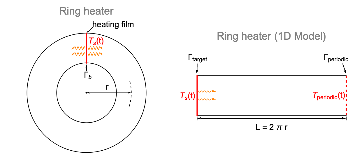
As an example a ring heater is modeled where a thin film is inserted to serve as a heat source. It is possible to perform the simulation with a 1D domain by using the periodic boundary condition.
The ring heater is converted into a 1D model with the length ![]() which is the perimeter of the ring. To simulate the heating process the temperature
which is the perimeter of the ring. To simulate the heating process the temperature ![]() of the heating film is specified at the left boundary. At the right hand boundary
of the heating film is specified at the left boundary. At the right hand boundary ![]() a periodic boundary condition is applied to map the boundary temperature
a periodic boundary condition is applied to map the boundary temperature ![]() to the target boundary
to the target boundary ![]() .
.
Here a smoothed step function is used to prescribe a temperature profile ![]() on the heating film. The parameters
on the heating film. The parameters ![]() and
and ![]() are chosen arbitrarily to fit the parameters of heat transfer model.
are chosen arbitrarily to fit the parameters of heat transfer model.
The simulation begins with an undisturbed domain where ![]() . During the heating process, the temperature
. During the heating process, the temperature ![]() on the periodic boundary has been mapped to the left hand boundary while the temperature
on the periodic boundary has been mapped to the left hand boundary while the temperature ![]() of the heating film increases. The thermal energy is then transferred from both ends and gradually heats up the domain.
of the heating film increases. The thermal energy is then transferred from both ends and gradually heats up the domain.
As an alternative in this example the PeriodicBoundaryCondition could be replaces by using the DirichletCondition from the left boundary also at the right boundary
It is also worth noting that if the left hand side had been any other boundary condition, the PeriodicBoundaryCondition would have projected that to the right. In other words the PeriodicBoundaryCondition projects whatever boundary condition it finds to the target.
Appendix
Special Cases of the Heat Equation
If the temperature field is in a steady state, the transient term in (42) vanishes and the heat equation simplifies to:
When modeling a heat transfer problem, sometimes it is not convenient to describe the model in Cartesian coordinates ![]() . The heat equation may also be expressed using a cylindrical or spherical coordinate system.
. The heat equation may also be expressed using a cylindrical or spherical coordinate system.
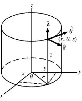
A graphics showing cylindrical coordinates:
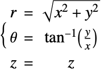
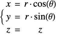
In the cylindrical coordinate system ![]() ,
, ![]() and
and ![]() denote the radial, azimuthal and vertical directions, respectively. In terms of the Cartesian coordinates
denote the radial, azimuthal and vertical directions, respectively. In terms of the Cartesian coordinates ![]() , the cylindrical coordinates are defined by:
, the cylindrical coordinates are defined by:
By inserting the coordinates relation (43) into (44), the heat equation can be expressed in cylindrical coordinates as:
If the heat transfer within a model is rotationally symmetric about the ![]() axis, the resulting temperature field
axis, the resulting temperature field ![]() will be invariant in the
will be invariant in the ![]() direction. The equation (45) then simplifies to:
direction. The equation (45) then simplifies to:
In that case, a 3D heat transfer problem can be modeled in a 2D domain by making use of this symmetric property. This type of model is known as an axisymmetric model. Examples of making use of the cylindrical coordinate system with a 2D axisymmetric model can be founded in the separate Heat Transfer Verification Tests notebook: one time independent 2D example and one time dependent 2D example.
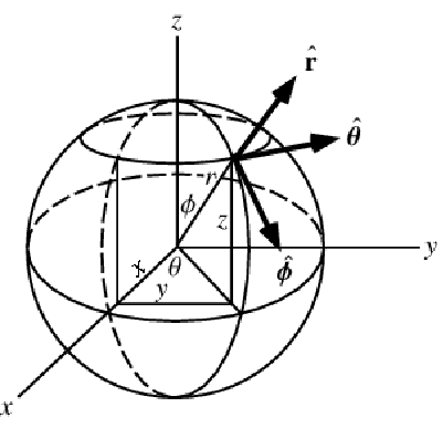
A graphics showing spherical coordinates:
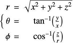
In the spherical coordinate system ![]() ,
, ![]() and
and ![]() denote the radial, azimuthal and polar directions, respectively. In terms of the Cartesian coordinates:
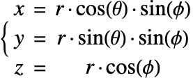
denote the radial, azimuthal and polar directions, respectively. In terms of the Cartesian coordinates: ![]() , the spherical coordinates are defined by:
, the spherical coordinates are defined by:
By inserting the coordinates relation (46) into (47), the heat equation can be expressed in the spherical coordinate system as:
The Smoothing Characteristic of the Diffusion Equation
The basic behaviour of a diffusion equation is smoothing. To see the effect set up initial conditions that are discontinuous at ![]() .
.
In a short time the sharp tip of the discontinuous initial condition at x=1/2 has been smoothed out. This smoothing effect is a major characteristic of the diffusion equation and therefore also of the heat equation.
Modeling Heat Sources using Element Markers
The most accurate and efficient method to deal with heat sources is by making use of element markers as then the mesh will have a specific subregion for the heat source which will result in an accurate solution. Element marker and their use in meshes is explained in detail in the section Element Marker in the Element Mesh Generation tutorial.
In the following 2D example we introduce a rectangular heat source ![]() to heat up the domain.
to heat up the domain.
Next we specify region markers with the "RegionMarker" option for ToElementMesh. To do so a coordinate within the heat source should be given, as well as an integer marker. Optionally, an additional maximum cell measure can be specified to refine the source region.
An alternative to generate the mesh is to make use of the Boolean region functions and specify the no region holes should be inserted. The same region marker process from above is used.
See this note about improving the visual quality of the animation.
This result agrees with the one that didn't make use of element makers, which is shown in the section: Volumetric Heat Source. For large complicates geometries the use of region element markers will be easier to set up and compute the solution more efficiently.
Conservation Laws with Discontinuous PDE coefficients
To explain why the heat transfer PDE holds for discontinuous density/velocity field, we start with the mass conservation:
Assume that the density ![]() and the flow velocity
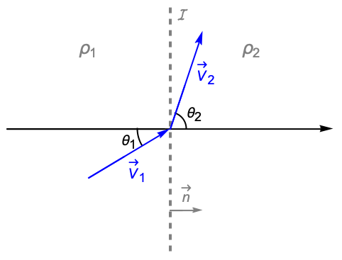
and the flow velocity ![]() are discontinuous at the interface ℐ:
are discontinuous at the interface ℐ:
Since there is no mass creation or destruction on the interface ℐ, the mass flux should still be the same on both sides of ℐ:
That is, the mass flux ![]() should be continuous throughout the domain. We can then apply the divergence theorem [48] on the equation (49) leading to:
should be continuous throughout the domain. We can then apply the divergence theorem [48] on the equation (49) leading to:
Since the domain ![]() is completely arbitrary, we can discard the integral and yield the mass conservation equation in the differential form:
is completely arbitrary, we can discard the integral and yield the mass conservation equation in the differential form:
That means the mass conservation equation (50) also holds true for the domain with discontinuous density/velocity field.
The heat equation is essentially an energy conservation equation, and can be derived in a similar way by substituting the density ![]() in (51) with the internal energy
in (51) with the internal energy ![]() . Therefore, the heat transfer model presented in the tutorial can be applied on both continuous and discontinuous density/velocity fields.
. Therefore, the heat transfer model presented in the tutorial can be applied on both continuous and discontinuous density/velocity fields.
Possible Issues and Workarounds for Modeling Heat Pulses
In the section: Heat Transfer with Events, we mentioned that it is possible to use an If statement to model heat pulses with time-dependent heat transfer model. However, when pulse durations become very small, the default time-stepping algorithm of NDSolve may fail to detect the prescribed heat pulse.
In the following section we will demonstrate the issue with an example, followed by two workarounds for modeling heat pulses.
Consider a 1D time-dependent heat transfer model with periodic heat pulses applied in the middle part of the domain. During time ![]() there are a total of five pulses with a duration of
there are a total of five pulses with a duration of ![]() .
.
To model the cooling of the domain, the temperature at both ends are fixed at ![]() .
.
For the demonstration purpose the thermal conductivity ![]() , the density
, the density ![]() and the heat capacity
and the heat capacity ![]() are set to one.
are set to one.
Note that without using options, NDSolve missed the last two heat pulses at ![]() and
and ![]() .
.
Next we present two possible workarounds to deal with this issue.
The first method is to specify a smaller time step for the time integration process by NDSolve. The option "MaxStepFraction" allows user to set the maximum fraction of the total time range to cover in a single step.
With a smaller time step NDSolve successfully captured all five heat pulses during ![]() .
.
Another, better, approach is to use WhenEvent to specify the heat pulses. The use of WhenEvent has the distinct advantage that NDSolve has special mechanisms build in to detect the pulses during the time integration. This mechanism may not be available when modeling heat pulses with an If or similar statement.
More details about the usage of WhenEvent and its event detection method can be found here.
In this approach the heat pulses is treated as a discrete variable ![]() by NDSolve, that is, it only changes at discrete times during the time integration. Note also, that not time integration step size reduction is necessary to obtain a solution.
by NDSolve, that is, it only changes at discrete times during the time integration. Note also, that not time integration step size reduction is necessary to obtain a solution.
With the usage of WhenEvent, NDSolve successfully captured all five heat pulses during ![]() .
.
Nomenclature
References
1. Bilbao, Stefan and Hamilton, Brian. Directional Source Modeling In Wave-Based Room Acoustics Simulation. IEEE, 2017.
2. Peskin, Charles. The Immersed Boundary Method. Cambridge University, 2002.
3. Churchill, Stuart W. and Chu, Humbert H.S. Correlating equations for laminar and turbulent free convection from a vertical plate. International Journal of Heat and Mass Transfer, 18 (11): 1323–1329, 1975.
4. Sukhatme, S.P. A Textbook on Heat Transfer (Fourth ed.). Universities Press. pp. 257–258, 2005.
5. Riedl, M. Optical Design Fundamentals for Infrared Systems (Second ed.). SPIE Press, Bellingham, WA, 2001.
6. Holman, J. P. Heat Transfer Tenth Edition, McGraw-Hill. pp. 111, Example 3-10 (2008).
7. Weisstein, Eric W. Divergence Theorem, MathWorld-A Wolfram Web Resource. http://mathworld.wolfram.com/DivergenceTheorem.html.
8. Onsager, L. Physical Review. 37, 405–426, (1931); 38, 2265–2279, (1931).
9. Casimir, H. B. G. Reviews of Modern Physics. 17, 343–350, (1945).
10. Hahn, D. W. and Özişik, M. N. Heat Conduction, John Wiley & Sons, Inc, ch.15 (2012).
