Events and Discontinuities in Differential Equations
| Introduction | Events and Discontinuous Differential Equations |
| Event Detection and Location | Examples |
| Event Actions |
Introduction
Differential equations alone are very effective for modeling continuous behavior of systems. However, many real systems involve components that change at discrete times, possibly triggered by states of the continuous solutions. For example, in a heating system, a thermostat will switch on once the temperature reaches a certain level.
An event trigger for a differential or differential algebraic system
is a point ![]() along the solution at which a Boolean-valued event function becomes True:
along the solution at which a Boolean-valued event function becomes True:
When ![]() is True for
is True for ![]() , then the value of
, then the value of ![]() can be found numerically during integration by evaluating
can be found numerically during integration by evaluating ![]() with an approximation of the solution and using bisection.
with an approximation of the solution and using bisection.
In general, much more robust and faster ways of numerically finding the value ![]() are available if
are available if ![]() is of the form
is of the form ![]() , where
, where ![]() is a real-valued function. Symbolic processing is automatically done on the event expression to try to get a real-valued function or simpler form if possible. For example, the Boolean event
is a real-valued function. Symbolic processing is automatically done on the event expression to try to get a real-valued function or simpler form if possible. For example, the Boolean event ![]() is specially processed so that an event will trigger at time
is specially processed so that an event will trigger at time ![]() , and the Boolean event
, and the Boolean event ![]() is automatically processed to the real function
is automatically processed to the real function ![]() .
.
For some event actions, such as discontinuity crossings, it is necessary to find a bracketing interval ![]() such that
such that ![]() is False and
is False and ![]() is True, or for a real-valued function
is True, or for a real-valued function ![]() , the signs of
, the signs of ![]() and
and ![]() are opposite.
are opposite.
When an event trigger is found, typically some action is performed. In some cases, the action can affect the integration of the system, by stopping integration or even changing the values of the solution variables, so the use of events in modeling gives a great deal of flexibility for discrete actions.
In NDSolve, events augment the differential equations with WhenEvent expressions.
| WhenEvent[event,action] | specify an action that occurs when the event triggers it for equations in NDSolve |
This section shows basic examples using WhenEvent in NDSolve. Subsequent sections in the tutorial go into more depth on topics including event detection and location, actions that modify state variables, discontinuity handling, and application examples.
Needs["DifferentialEquations`NDSolveProblems`"];
Needs["DifferentialEquations`NDSolveUtilities`"];
Needs["DifferentialEquations`InterpolatingFunctionAnatomy`"];
A simple example is locating an event, such as when a pendulum started at a nonequilibrium position will swing through its lowest point, and stopping the integration at that point.
sol = NDSolve[{y''[t] + Sin[y[t]] == 0, y'[0] == 0, y[0] == 1, WhenEvent[y[t] == 0, "StopIntegration"]}, y, {t, 0, 10}]From the solution you can see that the pendulum reaches its lowest point ![]() at about
at about ![]() . Using the InterpolatingFunctionAnatomy package, it is possible to extract the value from the InterpolatingFunction object.
. Using the InterpolatingFunctionAnatomy package, it is possible to extract the value from the InterpolatingFunction object.
end = InterpolatingFunctionDomain[First[y /. sol]][[1, -1]];
Plot[Evaluate[{y[t], y'[t]} /. First[sol]], {t, 0, end}, PlotStyle -> {{Green}, {Blue}}]
Event Detection and Location
Event location works in effectively two stages. In the event detection stage, for each time step taken by the numerical integration method each event is tested to see if it may have changed during the step. Once a possible event is detected, the location stage typically uses a root-finding procedure to find the actual event time ![]() .
.
Event Detection Methods
The simplest and fastest method for detecting whether an event occurred in a time step is to check for a change in the event function from False to True, or if it can be expressed as the root of a real function, a sign change.
The problem with just using the sign is that if a method takes large steps (such as extrapolation methods tend to) or the event function varies rapidly compared to the solution of the ODE, it is quite possible to miss events when double (or more) roots occur within a time step.
For events that can be expressed as a root of a real function, the method of using signs can be enhanced by including the time derivatives of the event function at the beginning and end of the step. For an ODE ![]() with event function
with event function ![]() , the time derivative is computed with
, the time derivative is computed with
The values can be interpolated by a cubic Hermite polynomial that can be tested to see if it has any roots in the step interval. If necessary, the step is subdivided so that a root can be bracketed for the root-finding procedure.
Using the derivative makes the detection more robust with relatively little extra cost if ![]() does not depend on
does not depend on ![]() , so this is the default method for those cases. However, it is still entirely possible that events can be omitted using this method.
, so this is the default method for those cases. However, it is still entirely possible that events can be omitted using this method.
For some problems, it is vital to ensure that events are not missed, and NDSolve supports a method using interpolation that is very robust, but it can be significantly more expensive. This method is based on using the continuous or dense output from the method to create an interpolant of the event function with the same order as the method. The interpolant is tested for roots in the time step using interval arithmetic techniques.
The method for event detection is controlled by the "EventDetection" option of WhenEvent.
| "Sign" | detect events from sign changes |
| "DerivativeSign" | additionally use the time derivative of the event function |
| "Interpolation" | interpolate the event function with a polynomial with the same order as the method |
Settings for the "DetectionMethod" option.
When the event function varies much more rapidly than the solutions of the differential equation itself, the time steps may include many crossings of an event function. This can be mitigated by including the event function in the system as a dependent variable, using the equation for the time derivative of the event shown above. This can be done automatically using the option setting "IntegrateEvent"->True in WhenEvent.
When the event is integrated, the event interpolation is even more robust, since the event function interpolant is just a component of the dense output of the time integration method. In this case, the roots of the interpolant are the event locations to the full accuracy of the method, so there is no need for using a general root-finding method. For this reason, with "DetectionMethod"->"Interpolation", the event is integrated by default.
Event Location Methods
Once an event has been detected, the next task is to refine the location of the time within the time step where the event occurs. There are several different methods that can be used to refine the position. These include simply taking the solution at the beginning or the end of the integration interval, a linear interpolation of the event value, and using bracketed root-finding methods. The appropriate method to use depends on a trade-off between execution speed and location accuracy.
The method used to refine the location is controlled by the "LocationMethod" option of WhenEvent.
| "Brent" | use FindRoot with Method->"Brent" to locate the event; this is the default with the setting Automatic |
| "BrentBracketRoot" | give the event handler a refined bracket for the root that is useful for discontinuity crossings |
| "LinearInterpolation" | locate the event time using linear interpolation; cubic Hermite interpolation is then used to find the solution at the event time |
| "StepBegin" | the event is given by the solution at the beginning of the step |
| "StepEnd" | the event is given by the solution at the end of the step |
Settings for the "LocationMethod" option.
Location of a single event is usually fast enough so that the method used will not significantly influence the overall computation time. However, when an event is detected multiple times, the location refinement method can have a substantial effect.
"StepBegin" and "StepEnd" Methods
The crudest methods are appropriate for when the exact position of the event location does not really matter or does not reflect anything with precision in the underlying calculation.
Here is an example where "StepEnd" is appropriate because the location of the event is arbitrary.
Button["Stop", stop = True]stop = False;usol = NDSolveValue[{D[u[t, x], t, t] == D[u[t, x], x, x], u[0, x] == Exp[-10 x ^ 2], Derivative[1, 0][u][0, x] == 0, u[t, -10] == u[t, 10], WhenEvent[stop, "StopIntegration"]}, u, {t, 0, 100}, {x, -10, 10}, Method -> "StiffnessSwitching"]In this example, time steps are computed so quickly that there is no way that you can time the click of a button to be within a particular time step, much less at a particular point within a time step. Thus, based on the inherent accuracy of the event, there is no point in refining at all, so it is most appropriate to use the "StepBegin" or "StepEnd" location methods. In any example where the definition of the event is heuristic or somewhat imprecise, this is the best appropriate choice.
"LinearInterpolation" Method
When event results are needed for the purpose of points to plot in a graph, you only need to locate the event to the resolution of the graph. While just using the step end is usually too crude for this, a single linear interpolation based on the event function values suffices.
Denote the event function values at successive mesh points of the numerical integration:
A linear approximation of the event time is then:
Linear interpolation could also be used to approximate the solution at the event time. However, since derivative values ![]() and
and ![]() are available at the mesh points, a better approximation of the solution at the event can be computed cheaply using cubic Hermite interpolation as
are available at the mesh points, a better approximation of the solution at the event can be computed cheaply using cubic Hermite interpolation as
for suitably defined interpolation weights:
You can specify refinement based on a single linear interpolation with the setting "LinearInterpolation".
lsol = NDSolveValue[{y''[t] + Sin[y[t]] == 0, y[0] == 3, y'[0] == 0, WhenEvent[y'[t] < 0, {lend = t, "StopIntegration"}, "LocationMethod" -> "LinearInterpolation"]}, y, {t, 0, ∞}, Method -> "ExplicitRungeKutta"];
Plot[{lsol[t], lsol'[t]}, {t, 0, lend}]
At the resolution of the plot over the entire period, you cannot see that the endpoint may not be exactly where the derivative hits the axis. However, if you zoom in enough, you can see the error.
Plot[lsol'[t], {t, end * (1 - .001), end * (1 + .001)}, PlotStyle -> Blue, PlotRange -> All, Epilog -> {PointSize[.025], Point[{end, 0}]}]The linear interpolation method is sufficient for most viewing purposes, such as computing Poincaré sections. Note that for Boolean-valued event functions, linear interpolation is effectively only one bisection step, so the linear interpolation method may be inadequate for graphics.
Brent's Method
The default location method is the event location method "Brent", finding the location of the event using FindRoot as described in "Brent's Method". Brent's method starts with a bracketed root and combines steps based on interpolation and bisection, guaranteeing a convergence rate at least as good as bisection and in most cases much better. You can control the accuracy and precision to which FindRoot tries to get the root of the event function using method options for the "Brent" event location method. The default is to find the root to the same accuracy and precision as NDSolve is using for local error control.
When the event depends on the solutions ![]() of the differential equation, the argument
of the differential equation, the argument ![]() needs to be approximated for
needs to be approximated for ![]() within the time step. For methods that support continuous or dense output, the argument for the event function can be found quite efficiently simply by using the continuous output formula. However, for methods that do not support continuous output, the solution needs to be computed by taking a step of the underlying method, which can be relatively expensive. An alternate way of getting a solution approximation that is not accurate to the method order, but is consistent with using FindRoot on the InterpolatingFunction object returned from NDSolve, is to use cubic Hermite interpolation, obtaining approximate solution values in the middle of the step by interpolation based on the solution values and solution derivative values at the step ends.
within the time step. For methods that support continuous or dense output, the argument for the event function can be found quite efficiently simply by using the continuous output formula. However, for methods that do not support continuous output, the solution needs to be computed by taking a step of the underlying method, which can be relatively expensive. An alternate way of getting a solution approximation that is not accurate to the method order, but is consistent with using FindRoot on the InterpolatingFunction object returned from NDSolve, is to use cubic Hermite interpolation, obtaining approximate solution values in the middle of the step by interpolation based on the solution values and solution derivative values at the step ends.
For events that are set up to handle discontinuity crossings, it is very useful for the event handler to have a bracketing interval ![]() so that it can do proper evaluations on either side of the discontinuity and ensure the crossing is done correctly. This is done with the method "BrentBracketRoot".
so that it can do proper evaluations on either side of the discontinuity and ensure the crossing is done correctly. This is done with the method "BrentBracketRoot".
Method options can be passed to the "Brent" and "BrentBracketRoot" methods that control the solution approximation and the use of FindRoot.
option name | default value | |
| "MaxIterations" | 100 | the maximum number of iterations to use |
| "AccuracyGoal" | Automatic | accuracy goal setting passed to FindRoot |
| "PrecisionGoal" | Automatic | precision goal setting passed to FindRoot |
| "SolutionApproximation" | Automatic | how to approximate the solution for evaluating the event function during the refinement process; can be Automatic or "CubicHermiteInterpolation" |
Options for event location methods "Brent" and "BrentBracketRoot".
If the AccuracyGoal or PrecisionGoal settings are Automatic, the value passed to FindRoot is based on the local error setting for NDSolve.
Location Method Comparison
This example integrates the pendulum equation for a number of different event location methods and compares the time when the event is found.
eventmethods = {"StepBegin", "StepEnd", "LinearInterpolation", Automatic};Map[
NDSolve[{y''[t] + Sin[y[t]] == 0, y[0] == 3, y'[0] == 0, WhenEvent[y'[t] < 0, {Print[#, ": t = ", t, " y'[t] = ", y'[t]], "StopIntegration"}, "LocationMethod" -> #]}, y, {t, 0, ∞}, Method -> "ExplicitRungeKutta"]&,
eventmethods
];Event Actions
With WhenEvent[event,action], once an event trigger point ![]() is detected and located along a solution trajectory, then the event handler evaluates the action given in the second argument of WhenEvent.
is detected and located along a solution trajectory, then the event handler evaluates the action given in the second argument of WhenEvent.
First, the solution values ![]() are approximated, typically using a dense output formula for the time integration method. The derivatives
are approximated, typically using a dense output formula for the time integration method. The derivatives ![]() are found by evaluating the right-hand side function for ODEs or using the dense output formula for DAEs. Then (in a way similar to Block) the time-independent variable is set to
are found by evaluating the right-hand side function for ODEs or using the dense output formula for DAEs. Then (in a way similar to Block) the time-independent variable is set to ![]() and the dependent variables and their derivatives are set to the approximate values in
and the dependent variables and their derivatives are set to the approximate values in ![]() and
and ![]() , and the expression is evaluated. If the value returned from the evaluation is a Rule or a string directive, then the event handler will execute the directed action.
, and the expression is evaluated. If the value returned from the evaluation is a Rule or a string directive, then the event handler will execute the directed action.
| "StopIntegration" | stop integrating at |
| "RestartIntegration" | restart the integration at |
| "CrossDiscontinuity" | integrate to |
| "CrossSlidingDiscontinuity" | integrate to |
| "RemoveEvent" | remove the event |
| y[t]->val | change the state variable y to val |
| d[t]->"DiscontinuitySignature" | change the discontinuity signature variable d |
With WhenEvent[event,{action1,action2,…}], actioni is evaluated and handled completely before actioni+1 is evaluated, so it is possible to give a sequence of actions that will be triggered for a single event.
There are many examples of event actions with and without directives in the reference page for WhenEvent. A few examples are given here that illustrate the sequential evaluation and the handling of directives.
{sol, data} = Reap[NDSolve[{x'[t] == y[t], y'[t] == -t x[t], x[0] == 1, y[0] == 1, WhenEvent[x[t] == y[t], Sow[{t, x[t]}];If[Abs[x[t]] < 1, "StopIntegration"]]}, {x, y}, {t, ∞}]]tend = data[[1, -1, 1]];
Plot[Evaluate[{x[t], y[t]} /. sol], {t, 0, tend}, Epilog -> {PointSize[0.05], Red, Apply[Point, data]}]Changing State Variables
In general, evaluation of an arbitrary action expression does not affect the solution state variables that are used by NDSolve. Using an action in WhenEvent that evaluates to a rule provides a flexible way of making state changes at a discrete event time.
A simple example of this is a model of a ball bouncing elastically on a flat surface.
g = 9.8; r = .95;
bb = NDSolveValue[{x''[t] == -g, x[0] == 1, x'[0] == 0, WhenEvent[x[t] == 0, x'[t] -> -r x'[t]]}, x, {t, 0, 5}];
Plot[bb[t], {t, 0, 5}]
The rule x'[t]->-r x[t] specifies that the state variable x′[t] is replaced with -r x′[t] whenever x[t]0. After the change is made, the integration is restarted, since effectively a new solution trajectory is being computed.
A change for several state variables can be specified either using a single rule with a list of variables and values or multiple rules. There are subtle semantic differences between the two approaches, demonstrated by the examples below.
Δt = 3;T = 20;
sol = First[NDSolve[{x'[t] == y[t], y'[t] +   y[t] + 2 x[t] == 0, x[0] == 0, y[0] == 1, WhenEvent[Mod[t, Δt] == 0, {x[t], y[t]} -> {4 y[t], x[t]}]}, {x, y}, {t, 0, T}]];
ParametricPlot[Evaluate[{x[t], y[t]} /. sol], {t, 0, T}, PlotRange -> All]
In the rule {x[t],y[t]}->{y[t],x[t]}, the right-hand side is evaluated and then the corresponding state variables are set. When the action is a list of rules, each rule is evaluated in turn.
sol2 = First[NDSolve[{x'[t] == y[t], y'[t] +   y[t] + 2 x[t] == 0, x[0] == 0, y[0] == 1, WhenEvent[Mod[t, Δt] == 0, {x[t] -> 4 y[t], y[t] -> x[t]}]}, {x, y}, {t, 0, T}]];
ParametricPlot[Evaluate[{x[t], y[t]} /. sol2], {t, 0, T}, PlotRange -> All]
With the two rules, first ![]() is set to
is set to ![]() and then
and then ![]() is set to the new value of
is set to the new value of ![]() , so the second rule actually has the effect of setting
, so the second rule actually has the effect of setting ![]() to
to ![]() .
.
For an ODE system ![]() , it is not possible to set the derivatives x'[t], since those are determined explicitly from the function. For higher-order systems that are automatically reduced to first order, this means that the highest-order derivative that appears in the equations cannot be set.
, it is not possible to set the derivatives x'[t], since those are determined explicitly from the function. For higher-order systems that are automatically reduced to first order, this means that the highest-order derivative that appears in the equations cannot be set.
Δt = 3;T = 20;
dsol = First[NDSolve[{x'[t] == y[t], y'[t] +   y[t] + 2 x[t] == 0, x[0] == 0, y[0] == 1, WhenEvent[Mod[t, Δt] == 0, {x'[t], y'[t]} -> {4 y[t], x[t]}]}, {x, y}, {t, 0, T}]];
ParametricPlot[Evaluate[{x[t], y[t]} /. dsol], {t, 0, T}, PlotRange -> All]
When solving as a system of differential-algebraic equations ![]() , it is possible to set the derivatives. A part of the DAE solving process is to find consistent values
, it is possible to set the derivatives. A part of the DAE solving process is to find consistent values ![]() and
and ![]() so that the residual
so that the residual ![]() is 0. NDSolve is directed to treat equations as a system of DAEs if you use the Method option setting Method->{"EquationSimplification"->"Residual"}.
is 0. NDSolve is directed to treat equations as a system of DAEs if you use the Method option setting Method->{"EquationSimplification"->"Residual"}.
Δt = 3;T = 20;
daesol = First[NDSolve[{x'[t] == y[t], y'[t] +   y[t] + 2 x[t] == 0, x[0] == 0, y[0] == 1, WhenEvent[Mod[t, Δt] == 0, {x'[t], y'[t]} -> {4 y[t], x[t]}]}, {x, y}, {t, 0, T}, Method -> {"EquationSimplification" -> "Residual"}]];
ParametricPlot[Evaluate[{x[t], y[t]} /. daesol], {t, 0, T}, PlotRange -> All]
When either the variables or their derivatives are changed when solving as a DAE of the form ![]() , unless the new values given satisfy
, unless the new values given satisfy ![]() , a reinitialization needs to be computed where an attempt is made to find values of the variables that were not changed, so that
, a reinitialization needs to be computed where an attempt is made to find values of the variables that were not changed, so that ![]() . Details of the procedure and examples are given in "DAE Reinitialization with Events".
. Details of the procedure and examples are given in "DAE Reinitialization with Events".
When the action is not explicitly a rule, the action is evaluated after replacing all explicit instances of Rule in the action expression with a special private head that has the attribute HoldFirst, so that the states on the left-hand side do not evaluate. If the return value has this special head, then a state change is executed.
Δt = 1;
xsols = Table[NDSolveValue[{x''[t] + x'[t] + x[t] == Cos[t], x[0] == x'[0] == 0, WhenEvent[Mod[t, Δt] == 0, If[RandomChoice[{1 / 3, 2 / 3} -> {True, False}], x[t] -> -x[t]]]}, x[t], {t, 0, 10}], {10}];
Plot[Evaluate[xsols], {t, 0, 10}]
Discrete variables specified with the DiscreteVariables option can only be changed through rules. An advantage of using discrete variables is that they do not increase the system size that the differential equation solver methods work with—this is particularly important for stiff methods where the Jacobian is used.
Events and Discontinuous Differential Equations
The methods built into NDSolve for solving systems of differential equations are all effectively based on an implicit assumption that the differential equation satisfies some basic continuity conditions. For ODEs, a sufficient condition is Lipschitz continuity.
When a differential equation has discontinuities, these assumptions are violated and solvers may get poor quality solutions or, in some cases, may not be able to find solutions at all. Typically what happens is that in an attempt to satisfy local error tolerances, the solvers decrease step size until the step is so small that error tolerances appear to be satisfied even with the discontinuous function values, and the solver continues beyond the discontinuity with the approximation it found.
As an example, consider the ODE
f1[a_][t_, x_] = t^2 + 2 x^2;
f2[a_][t_, x_] = 2t^2 + 3 x^2 - a;
f[a_][t_, x_] = If[(x + (3/20))^2 + (t + (1/20))^2 ≤ 1, f1[a][t, x], f2[a][t, x]];fb[a_][t_ ? NumberQ, x_] := f[a][t, x];opts = {Method -> {"TimeIntegration" -> {"ExplicitRungeKutta", "DifferenceOrder" -> 7}}};Block[{s = 0}, bsol = NDSolveValue[{x'[t] == fb[2][t, x[t]], x[0] == 3 / 10}, x, {t, 1}, StepMonitor :> s++, opts];s]ListLinePlot[bsol, Mesh -> All, PlotRange -> All]The solution shown here was computed without any a priori knowledge of the discontinuity, and the reduction to the time step just prior to the discontinuity is seen. Once the discontinuity has been crossed, the time steps increase in size again. Essentially the same thing happens with the default (multistep) method, but a higher-order Runge–Kutta method was chosen for this example to emphasize the effect.
If the time at which a discontinuity is encountered can be identified, then an alternative way of handling the discontinuity is to step up to the discontinuity using values from the approaching side and then restart the integration using values on the other side of the discontinuity. Both the extremely small time steps and possible errors can be avoided this way.
A natural way of identifying the time at which a discontinuity is encountered is to set up an event. In the Wolfram Language, this can be done with WhenEvent. One issue with using events to detect discontinuities is that for events that depend on the solution, the solution may need to be computed past the event to correctly locate the event, but that involves the approximation of the solution across the discontinuity the event was set up to avoid in the first place. NDSolve avoids this problem by using discontinuity signature discrete variables that are only switched when the discontinuity is encountered, so that the solver in effect samples a smooth function. This is done automatically by NDSolve when it symbolically detects discontinuous functions in the differential equations, but it is possible to set up WhenEvent expressions explicitly that do the same thing; details are described following.
Block[{s = 0}, dsol = NDSolveValue[{x'[t] == f[2][t, x[t]], x[0] == 3 / 10}, x, {t, 1}, StepMonitor :> s++, opts];s]When NDSolve can see the symbolic form of the function, it is able to automatically identify the discontinuity and handle it using an event. This approach requires far fewer time steps.
x1[t_] = First[x[t] /. DSolve[{x'[t] == f1[2][t, x[t]], x[0] == 3 / 10}, x, t]];
switchpoint = t /. FindRoot[(x + (3/20))^2 + (t + (1/20))^2 == 1 /. {x -> x1[t]}, {t, .6}, WorkingPrecision -> 100];
x2[t_] = Block[{a = 2}, First[x[t] /. DSolve[{x'[t]  == f2[2][t, x[t]], x[s] == x1[s]}, x, t] /. s -> switchpoint]];
SetAttributes[x100, Listable];
x100[t_] := Re[Piecewise[{{x1[t], t ≤ switchpoint}}, x2[t]]];bsteps = Part[InterpolatingFunctionCoordinates[bsol], 1, 2 ;; -1];
dsteps = Part[InterpolatingFunctionCoordinates[dsol], 1, 2 ;; -1];ListLogPlot[{Map[{#, Abs[bsol[#] - x100[#]]}&, bsteps], Map[{#, Abs[dsol[#] - x100[#]]}&, dsteps]}, PlotRange -> All, Joined -> True]The error makes a jump of several orders of magnitude when the discontinuity is not handled using an event.
When the parameter ![]() is increased sufficiently, numerical methods without events are not generally able to continue past the discontinuity because when the discontinuity is first encountered, the solution on either side points back toward the discontinuity.
is increased sufficiently, numerical methods without events are not generally able to continue past the discontinuity because when the discontinuity is first encountered, the solution on either side points back toward the discontinuity.
Block[{s = 0}, bsol = NDSolveValue[{x'[t] == fb[5][t, x[t]], x[0] == 3 / 10}, x, {t, 1}, StepMonitor :> s++, opts];s]With ![]() , numerical methods without events are not generally able to continue past the discontinuity because when the discontinuity is first encountered, the solution on either side points back toward the discontinuity.
, numerical methods without events are not generally able to continue past the discontinuity because when the discontinuity is first encountered, the solution on either side points back toward the discontinuity.
Show[VectorPlot[{1, f[5][t, x]}, {t, .5, .7}, {x, .5, .7}, Prolog -> {Thickness[.015], Yellow, Circle[{-1 / 20, -3 / 20}]}, FrameLabel -> {t, x}], Plot[bsol[t], {t, .5, 0.6235830505886174}, PlotStyle -> Red]]Block[{s = 0}, dsol = NDSolveValue[{x'[t] == f[5][t, x[t]], x[0] == 3 / 10}, x, {t, 1}, StepMonitor :> s++, opts];s]ListLinePlot[dsol, Mesh -> All, PlotRange -> All, Prolog -> {Thickness[.015], Yellow, Circle[{-1 / 20, -3 / 20}]}, AxesLabel -> {t, x}]With the symbolic detection of the discontinuity, even though the Wolfram Language conditions for unique existence of the solution are violated, NDSolve is able to compute a continuation known as Filippov [F88] sliding mode in this situation. When the vector field points toward the discontinuity on both sides, the continuation effectively slides along the discontinuity surface until the field on one side or the other points away. This can be seen in the plot above where the solution is directly on the circle for some time, but eventually deviates.
The following sections of this tutorial explain the Filippov continuation and how to use discontinuity signatures.
Sliding Mode
When a discontinuity surface is encountered and the vector field on either side of the surface points back toward the solution, some sort of continuation method is necessary. Without a continuation, a numerical method will typically fail as it tries to take steps that cross and then recross the discontinuity; in some cases the numerical solution will display artificial chattering.
An appropriate continuation defined by Filippov [F88] effectively takes a convex combination of the components of the vector fields pointing along the discontinuity surface (or orthogonal to the gradient vector of a function for which the surface is a level curve).

In the preceding figure, the discontinuity surface is defined by ![]() and the vector fields for
and the vector fields for ![]() and
and ![]() are
are ![]() and
and ![]() , respectively. Then on the surface
, respectively. Then on the surface ![]() use
use ![]() , where
, where ![]() is chosen so that
is chosen so that ![]() is normal to the gradient
is normal to the gradient ![]() , in particular
, in particular ![]() . The solution can enter sliding mode either from above or below, as shown in the left and right parts of the figure, respectively.
. The solution can enter sliding mode either from above or below, as shown in the left and right parts of the figure, respectively.
The preceding definition is given for an autonomous system ![]() with no explicit dependence on the independent variable
with no explicit dependence on the independent variable ![]() . The same ideas apply for a nonautonomous system
. The same ideas apply for a nonautonomous system ![]() by adding a variable
by adding a variable ![]() and considering the autonomous system
and considering the autonomous system ![]() .
.
A simple example is provided by the vector field ![]() that has a discontinuity surface
that has a discontinuity surface ![]() . For this vector field
. For this vector field ![]() ,
, ![]() , and
, and ![]() ; therefore
; therefore ![]() , so
, so ![]() and the sliding motion is governed by
and the sliding motion is governed by ![]() .
.
vf = VectorPlot[{1, Sign[1 - y]}, {x, 0, 2}, {y, 0, 2}, VectorStyle -> Gray, VectorPoints -> 2.Flatten[Outer[List, Range[0, 11] / 11, Range[0, 11] / 11], 1]]fb[y_ ? NumberQ] := Sign[1 - y];
sol0 = First[NDSolve[{x'[t] == 1, y'[t] == fb[y[t]], x[0] == 0, y[0] == 2}, {x, y}, {t, 0, 2}]];ParametricPlot[Evaluate[{x[t], y[t]} /. sol0], {t, 1, 1.000036}, AspectRatio -> 1]The default method gets stuck because it eventually gets to tiny steps that chatter along the discontinuity.
fb[y_ ? NumberQ] := If[y > 1, -1, 1];
sole = First[NDSolve[{x'[t] == 1, y'[t] == fb[y[t]], x[0] == 0, y[0] == 2}, {x, y}, {t, 0, 2}, Method -> "Extrapolation"]];Show[vf, ParametricPlot[{x[t], y[t]} /. sole, {t, 0, 2}]]The solution shown above is not correct; the larger oscillation or chattering of the solution near the sliding surface is an artifact of the numerical method.
sol = First[NDSolve[{x'[t] == 1, y'[t] == Sign[1 - y[t]], x[0] == 0, y[0] == 2}, {x, y}, {t, 0, 2}]];Show[vf, ParametricPlot[Evaluate[{x[t], y[t]} /. sol], {t, 0, 2}]]When the discontinuous function is explicit in the equations, NDSolve can handle the discontinuity automatically by using the Filippov continuation.
The Filippov continuation is a natural choice since solving a sequence of systems with smooth functions approaching the discontinuous one approaches the sliding mode solution.
smooth[ϵ_][z_] := 2ArcTan[z / ϵ] / π
Plot[Evaluate[Table[smooth[10^k][z], {k, 0, -4, -1 / 4}]], {z, -1, 1}]Manipulate[Module[{ϵ = 10. ^ k, ϵsol},
ϵsol = First[NDSolve[{x'[t] == 1, y'[t] == smooth[ϵ][1 - y[t]], x[0] == 0, y[0] == 2}, {x, y}, {t, 0, 2}]];
Show[vf, ParametricPlot[Evaluate[{x[t], y[t]} /. {sol, ϵsol}], {t, 0, 2}]]], {{k, -1, "SubscriptBox[Log, 10][ϵ]"}, -4, 0}, SaveDefinitions -> True]In general, a trajectory will be trapped in sliding mode until one of the vector fields starts to point away. When this happens, the solution can be continued above or below the discontinuity.

In the figure above, the discontinuity surface is defined by ![]() and the vector fields for
and the vector fields for ![]() and
and ![]() are
are ![]() and
and ![]() , respectively. Then on the surface
, respectively. Then on the surface ![]() use
use ![]() , where
, where ![]() is chosen so that
is chosen so that ![]() is normal to the gradient
is normal to the gradient ![]() , in particular
, in particular ![]() . Beyond the point shown in both sides of the figure,
. Beyond the point shown in both sides of the figure, ![]() and
and ![]() both have the same sign. On the left
both have the same sign. On the left ![]() because
because ![]() and
and ![]() , and on the right
, and on the right ![]() because
because ![]() and
and ![]() , and in either case the trajectory exits sliding mode. These points can be found by numerically finding either the root
, and in either case the trajectory exits sliding mode. These points can be found by numerically finding either the root ![]() or
or ![]() as appropriate.
as appropriate.
Consider the vector field ![]() . Once
. Once ![]() , the vector field shown following starts to point down again, and the trajectory can escape sliding mode.
, the vector field shown following starts to point down again, and the trajectory can escape sliding mode.
sole = First[NDSolve[{x'[t] == 1, y'[t] == If[y[t] - 1 > 0, -1, 1 - x[t] / 2], x[0] == 0, y[0] == 2}, {x, y}, {t, 0, 3}]];Show[VectorPlot[{1, If[y > 1, -1, 1 - x / 2]}, {x, 0, 3}, {y, 0, 2}, VectorStyle -> Gray, VectorPoints -> Flatten[Outer[List, 3.Range[0, 16] / 16, 2.Range[0, 11] / 11], 1]], ParametricPlot[{x[t], y[t]} /. sole, {t, 0, 3}]]It may occur that a solution enters and exits sliding mode repeatedly.
Consider the vector field ![]() . For
. For ![]() , this is just an oscillator with negative damping. For
, this is just an oscillator with negative damping. For ![]() , all trajectories approach the discontinuity surface
, all trajectories approach the discontinuity surface ![]() . On
. On ![]() , if
, if ![]() is not too large, there is a set of points where there is sliding motion. The sliding motion in effect stabilizes the unbounded growth that would occur with the negative damping, and so there is a periodic orbit.
is not too large, there is a set of points where there is sliding motion. The sliding motion in effect stabilizes the unbounded growth that would occur with the negative damping, and so there is a periodic orbit.
Manipulate[Module[{x0, y0, sol},
	{x0, y0} = p; sol  =   First[NDSolve[{x'[t] == y[t], y'[t] == If[y[t] - 1 > 0, -1, .1 y[t] - x[t]], x[0] == x0, y[0] == y0}, {x, y}, {t, 0, 20}]];
	ParametricPlot[{x[t], y[t]} /. sol, {t, 0, 20}, PlotRange -> {{-1.5, 1.5}, {-1.5, 1.5}}]],
	{{p, {-1.5, 1.5}}, Locator}]
All of the examples shown so far are in two dimensions, since that is easier to visualize. However, the continuation works in any number of dimensions, and solutions can arise where the solution slides on more than one discontinuity surface at once.
Consider the two discontinuity surfaces in 3D defined by the surface of a sphere ![]() and the plane
and the plane ![]() and the vector field given by
and the vector field given by ![]() .
.
sol = First[NDSolve[{x'[t] == Sign[8 - y[t] ^ 2 - (x[t] + 3 / 2) ^ 2 - (z[t] - 1) ^ 2], y'[t] == Sign[-y[t]], z'[t] == 1,
	x[0] == 2, y[0] == -2, z[0] == 0}, {x, y, z}, {t, 0, 5}]]
Plot[Evaluate[{x[t], y[t], z[t]} /. sol], {t, 0, 5}, ImageSize -> Medium]c1 = ContourPlot3D[8 - y ^ 2 - (x + 3 / 2) ^ 2 - (z - 1) ^ 2, {x, -2, 2}, {y, -2, 2}, {z, 0, 5}, Contours -> 0, Mesh -> False];
c2 = ContourPlot3D[-y, {x, -2, 2}, {y, -2, 2}, {z, 0, 5}, Contours -> 0, Mesh -> False];p1 = ParametricPlot3D[Evaluate[{x[t], y[t], z[t]} /. sol], {t, 0, 5}, PlotStyle -> {Thickness[.015], Red}];
Show[c1, c2, p1, ImageSize -> Medium]The solution first slides along the surface of the sphere, then along both surfaces, and eventually just along the plane.
Discontinuity Signature
For functions with complicated definitions such that symbolic processing of discontinuities is not possible, it is possible to set up manually the same sort of discontinuity handling that NDSolve does automatically for discontinuous functions.
Discontinuity signature variables are set up by including a WhenEvent expression where the event is on the discontinuity surface, and the action is rule setting the variable to "DiscontinuitySignature" and using the DiscreteVariables option to specify the range of the variable to be either {-1,0,1} or {-1,1}.
| WhenEvent[e0,s[t]->"DiscontinuitySignature] | specify that the discrete variable s[t] holds the discontinuity signature of the discontinuity surface defined by e such that s[t] is effectively Sign[e] |
| DiscreteVariables->{s[t]∈{-1,0,1}} | indicate that s[t] is a discrete variable with possible values -1, 0, and 1; sliding mode solutions will be considered |
| DiscreteVariables->{s[t]∈{-1,1}} | indicate that s[t] is a discrete variable with possible values -1 and 1; sliding mode solutions will not be considered |
Setting up a discontinuity signature variable s[t].
Consider the first example in the previous section on sliding mode with the vector field ![]() .
.
sol = First[NDSolve[{x'[t] == 1, y'[t] == s[t], x[0] == 0, y[0] == 2, s[0] == -1, WhenEvent[1 - y[t] == 0, s[t] -> "DiscontinuitySignature"]}, {x, y, s}, {t, 0, 2}, DiscreteVariables -> s[t]∈{-1, 0, 1}]]Row[{ParametricPlot[{x[t], y[t]} /. sol, {t, 0, 2}, PlotRange -> {0, 2}]Plot[s[t] /. sol, {t, 0, 2}, PlotStyle -> Thickness[.02]]}]The variable ![]() switches from
switches from ![]() to 0 when the discontinuity is encountered and the solution goes into sliding mode. Sliding mode is indicated by a discontinuity signature of 0, since ideally the solution is exactly on the discontinuity surface
to 0 when the discontinuity is encountered and the solution goes into sliding mode. Sliding mode is indicated by a discontinuity signature of 0, since ideally the solution is exactly on the discontinuity surface ![]() and so
and so ![]() is 0. In practice, the actual solution may not satisfy this due to numerical error. When in sliding mode, NDSolve tries to keep as close to the surface as possible.
is 0. In practice, the actual solution may not satisfy this due to numerical error. When in sliding mode, NDSolve tries to keep as close to the surface as possible.
If you know that a discontinuity will not lead to sliding mode, the needed computations can be done less expensively if you exclude 0 from the range of the discontinuity signature variable. However, if you do this and there could be sliding mode on the discontinuity, the solution will fail or be incorrect.
sol = First[NDSolve[{x'[t] == 1, y'[t] == s[t], x[0] == 0, y[0] == 2, s[0] == -1, WhenEvent[1 - y[t] == 0, s[t] -> "DiscontinuitySignature"]}, {x, y, s}, {t, 0, 2}, DiscreteVariables -> s[t]∈{-1, 1}]]ParametricPlot[{x[t], y[t]} /. sol, {t, 0, 2}]An autonomous system defined by
can be represented by ![]() , where
, where ![]() is set by the Wolfram Language expression WhenEvent[e[x[t]]>0,s[t]->"DiscontinuitySignature"] in NDSolve.
is set by the Wolfram Language expression WhenEvent[e[x[t]]>0,s[t]->"DiscontinuitySignature"] in NDSolve.
The time derivative of the event function, ![]() is important in determining what happens when
is important in determining what happens when ![]() at some time
at some time ![]() . There are six cases where
. There are six cases where ![]() will be changed when
will be changed when ![]() with WhenEvent[e[x[t]]>0,s[t]->"DiscontinuitySignature"].
with WhenEvent[e[x[t]]>0,s[t]->"DiscontinuitySignature"].

Crossing from below and above.
- Case 1: (Cross from below)
 and
and  for
for  with
with 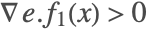 at
at  . The solution trajectory simply crosses to
  and
and  is set to
  .
.

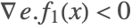
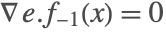
- Case 3: (Enter sliding mode from above)
 and
and  for
for  with
with 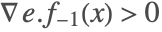 at
at  . Since
  is decreasing to zero it also holds that
 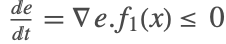 at
at  . The derivative
  is negative above and positive below the discontinuity, so the trajectory is trapped on the discontinuity. This is referred to as sliding mode and the value of
  is set to 0. The effective vector field
  is computed using the Filippov continuation
  , where
  . Note that
  since
since  and
and  .
.

- Case 5: (Exit sliding mode to above)
 ,
,  ,
,  , and
, and  for
for  and at
 with
with  . The solution is no longer in sliding mode and
  is set to 1. Note that the event that triggers this change is effectively a zero crossing of
 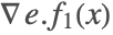 .
.
- Case 6: (Exit sliding mode to below)
 ,
,  ,
,  , and
, and  for
for  and at
 with
with 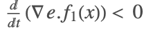 . The solution is no longer in sliding mode and
  is set to
  . Note that the event that triggers this change is effectively a zero crossing of
  .
.
To see all of these cases in an actual example, consider the system of ODEs
where ![]() and
and ![]() are constants that can be defined to see the different cases.
are constants that can be defined to see the different cases.
de[fa_, fb_] := {x'[t] == 1, y'[t] == (1/2)(1 + s[t])fa + (1/2)(1 - s[t])fb};solver[fa_, fb_][y0_] := First[NDSolve[{de[fa, fb] , x[0] == 0, y[0] == y0, s[0] == 0, WhenEvent[y[t] - 1 - Sin[π x[t]] / 4 == 0, s[t] -> "DiscontinuitySignature"]}, {x, y, s}, {t, 0, 2}, DiscreteVariables -> s[t]∈{-1, 0, 1}]];plotter[fa_, fb_][y0_] := Module[{sol, vf, psol, ps, sliding, g, α},
sol = solver[fa, fb][y0];
sliding = MemberQ[InterpolatingFunctionValuesOnGrid[s /. sol], 0.];
psol = ParametricPlot[Evaluate[{{x[t], y[t]} /. sol, {t, 1 + Sin[π t] / 4}}], {t, 0, 2}, PlotStyle -> {{Red, Thickness[.02]}, {Green}}, PlotRange -> {{0, 2}, {0, 2}}];
vf = VectorPlot[{1, If[y > 1 + Sin[π x] / 4, fa, fb]}, {x, 0, 2}, {y, 0, 2}, VectorStyle -> Gray, VectorPoints -> Flatten[Outer[List, 2.Range[0, 16] / 16, 2.Range[0, 11] / 11], 1], FrameLabel -> {"x", "y"}, Epilog -> Line[{{-1, 1}, {3, 1}}]];
ps = Plot[s[t] /. sol, {t, 0, 2}, PlotStyle -> Thickness[.02], AxesLabel -> {"t", If[sliding, "s,α", "s"]}, PlotRange -> {-1, 1}];
If[sliding,
g[x_, y_] = D[y - 1 - Sin[π x] / 4, {{x, y}}];
α[s_ /; s == 0, x_, y_] := ({1, fb}.g[x, y]) / ({0, fb - fa}.g[x, y]);
ps = Show[ps, Plot[α[s[t], x[t], y[t]] /. sol, {t, 0, 2}, PlotStyle -> Gray]]];
Row[{Show[vf, psol], " ", ps}]]plotter[2, 1][0]plotter[-1, -2][2]plotter[-1, 1][2]plotter[-1, 1][0]plotter[-1 / 4, 1][1]plotter[-1, 1 / 3][2]Examples
Falling Body
This system models a body falling under the force of gravity encountering air resistance (see [M04]).
sol = NDSolveValue[{y''[t] == -1 + y'[t] ^ 2, y[0] == 1, y'[0] == 0, WhenEvent[y[t] < 0, {tend = t, "StopIntegration"}]}, y, {t, 0, Infinity}]Show[Plot[sol[t], {t, 0, tend}, Frame -> True, Axes -> False, PlotStyle -> Blue],
Graphics[{{Green, Circle[{0, 1}, 0.025]}, {Red, Circle[{tend, sol[tend]}, 0.025]}}]]Period of the Van der Pol Oscillator
The Van der Pol oscillator is an example of an extremely stiff system of ODEs. The event locator method can call any method for actually doing the integration of the ODE system. The default method, Automatic, automatically switches to a method appropriate for stiff systems when necessary, so that stiffness does not present a problem.
vsol = NDSolve[{(|                                             |           |
| ------------------------------------------- | --------- |
| y1'[t] == y2[t]                              | y1[0] == 2 |
| y2'[t] == 1000 (1 - y1[t] ^ 2) y2[t] - y1[t] | y2[0] == 0 |), WhenEvent[Subscript[y, 2][t] < 0, "StopIntegration"]},
	{Subscript[y, 1], Subscript[y, 2]}, {t, 3000}]
By selecting the endpoint of the NDSolve solution, it is possible to write a function that returns the period as a function of ![]() .
.
vper[μ_ ? NumberQ] := Module[{per = $Failed},
	NDSolve[{(|                                          |           |
| ---------------------------------------- | --------- |
| y1'[t] == y2[t]                           | y1[0] == 2 |
| y2'[t] == μ (1 - y1[t] ^ 2) y2[t] - y1[t] | y2[0] == 0 |),
WhenEvent[Subscript[y, 2][t] < 0, {per = t, "StopIntegration"}]}, {}, {t, Max[100, 3 μ]}];per]vper[1000]LogLogPlot[vper[μ], {μ, 1, 1000}]Of course, it is easy to generalize this method to any system with periodic solutions.
Poincaré Sections
Using Poincaré sections is a useful technique for visualizing the solutions of high-dimensional differential systems.
For an interactive graphical interface see the package EquationTrekker.
The Hénon–Heiles System
Define the Hénon–Heiles system that models stellar motion in a galaxy.
system = GetNDSolveProblem["HenonHeiles"];
vars = system["DependentVariables"];eqns = {system["System"], system["InitialConditions"]}
The Poincaré section of interest in this case is the collection of points in the ![]() plane when the orbit passes through
plane when the orbit passes through ![]() .
.
Since the actual result of the numerical integration is not required, it is possible to avoid storing all the data in InterpolatingFunction by specifying the output variables list (in the second argument to NDSolve) as empty, or {}. This means that NDSolve will produce no InterpolatingFunction as output, avoiding storing a lot of unnecessary data. NDSolve does give a message NDSolve::noout warning there will be no output functions, but it can safely be turned off in this case, since the data of interest is collected from the event actions.
The linear interpolation event location method is used because the purpose of the computation here is to view the results in a graph with relatively low resolution. If you were doing an example where you needed to zoom in on the graph to great detail or to find a feature, such as a fixed point of the Poincaré map, it would be more appropriate to use the default location method.
peqns = {eqns, WhenEvent[Subscript[Y, 1][T] == 0, Sow[{Subscript[Y, 2][T], Subscript[Y, 4][T]}]]};data =
Reap[
NDSolve[peqns, {}, {T, 10000},
Method -> {"FixedStep", "StepSize" -> 0.25, "Method" -> {"ExplicitRungeKutta", "DifferenceOrder" -> 4}},
MaxSteps -> ∞];
];psdata = data[[-1, 1]];
ListPlot[psdata, Axes -> False, Frame -> True, AspectRatio -> 1]Since the Hénon–Heiles system is Hamiltonian, a symplectic method gives much better qualitative results for this example.
sdata =
	Reap[
	NDSolve[peqns, {}, {T, 10000},
	Method -> {"FixedStep", "StepSize" -> 0.25, "Method" -> {"SymplecticPartitionedRungeKutta", "DifferenceOrder" -> 4, "PositionVariables" -> {Subscript[Y, 1][T], Subscript[Y, 2][T]}}}, MaxSteps -> ∞];
];psdata = sdata[[-1, 1]];
ListPlot[psdata, Axes -> False, Frame -> True, AspectRatio -> 1]The ABC Flow
system = GetNDSolveProblem["ArnoldBeltramiChildress"];
eqs = system["System"];
vars = system["DependentVariables"];
icvars = vars /. T -> 0;Y1 = eqs; Y1[[2, 2]] = 0;Y1Y2 = eqs;Y2[[{1, 3}, 2]] = 0; Y2ImplicitMidpoint = {"ImplicitRungeKutta", "Coefficients" -> "ImplicitRungeKuttaGaussCoefficients", "DifferenceOrder" -> 2, "ImplicitSolver" -> {"FixedPoint", AccuracyGoal -> 10, PrecisionGoal -> 10, "IterationSafetyFactor" -> 1}};ABCSplitting = {"Splitting",
"DifferenceOrder" -> 2,
"Equations" -> {Y2, Y1, Y2},
"Method" -> {"LocallyExact", ImplicitMidpoint, "LocallyExact"}};psect[ics_] :=
Module[{reapdata},
reapdata =
Reap[
NDSolve[{eqs, Thread[icvars == ics], WhenEvent[Subscript[Y, 2][T] == 0, Sow[{Subscript[Y, 1][T], Subscript[Y, 3][T]}]]}, {}, {T, 1000},
Method -> {"FixedStep", "StepSize" -> 1 / 4, Method -> ABCSplitting}, MaxSteps -> ∞]
];
reapdata[[-1, 1]]
];data =
Mod[Map[psect, {{4.267682454609692, 0, 0.9952906114885919},
{1.6790790859443243, 0, 2.1257099470901704},
{2.9189523719753327, 0, 4.939152797323216},
{3.1528896559036776, 0, 4.926744120488727},
{0.9829282640373566, 0, 1.7074633238173198},
{0.4090394012299985, 0, 4.170087631574883},
{6.090600411133905, 0, 2.3736566160602277},
{6.261716134007686, 0, 1.4987884558838156},
{1.005126683795467, 0, 1.3745418575363608},
{1.5880780704325377, 0, 1.3039536044289253},
{3.622408133554125, 0, 2.289597511313432},
{0.030948690635763183, 0, 4.306922133429981},
{5.906038850342371, 0, 5.000045498132029}}],
2π];
ListPlot[data, ImageSize -> Medium]Bouncing Ball
This example is a generalization of an example in [SGT03]. It models a ball bouncing down a ramp with a given profile. The example is good for demonstrating how you can use multiple invocations of NDSolve with event location to model some behavior.
Reflection[k_, ramp_][{x_, xp_, y_, yp_}] := Module[{gramp, gp},
	gramp = -ramp'[x];
	If[Not[NumberQ[gramp]],
	Print["Could not compute derivative "];
	Throw[$Failed]];
	gramp = {-ramp'[x], 1};
	If[ gramp.{xp, yp} == 0,
	Print["No reflection"];
	Throw[$Failed]];
	gp = {1, -1} Reverse[gramp];
(k / (gramp.gramp)) (gp gp.{xp, yp} - gramp gramp.{xp, yp})]BouncingBall[k_, ramp_, {x0_, y0_}] :=
Module[{end, bounces, prange, xmin, xmax, ymin, ymax, xtraj, ytraj, prev = {x0, y0}},
bounces = Part[
Reap[Sow[{x0, y0}];{xtraj, ytraj} = NDSolveValue[{x''[t] == 0, x'[0] == 0, x[0] == x0, y''[t] == -9.8, y'[0] == 0, y[0] == y0, WhenEvent[y[t] < ramp[x[t]], {Sow[{x[t], y[t]}], If[Norm[prev - {x[t], y[t]}] < 10 ^ -3 && Norm[{x'[t], y'[t]}] < 10 ^ -3, end = t;"StopIntegration", prev = {x[t], y[t]}], {x'[t], y'[t]} -> Reflection[k, ramp][{x[t], x'[t], y[t], y'[t]}]}]}, {x, y}, {t, 0, 10}]], 2, 1];
prange = {{xmin, xmax}, {ymin, ymax}} = Outer[#2[bounces[[All, #1]]]&, {1, 2}, {Min, Max}];
Show[Plot[ramp[x], {x, xmin, xmax}, PlotRange -> prange, Epilog -> {PointSize[.025], Map[Point, bounces]}, AspectRatio -> (ymax - ymin) / (xmax - xmin)], ParametricPlot[{xtraj[t], ytraj[t]}, {t, 0, end}, PlotStyle -> Red]]]ramp[x_] := If[x < 1, 1 - x, 0];
BouncingBall[.7, ramp, {0, 1.25}]circle[x_] := If[x < 1, Sqrt[1 - x ^ 2], 0];
BouncingBall[.7, circle, {.1, 1.25}]wavyramp[x_] := If[x < 1, 1 - x + .05 Cos[11 Pi x], 0];
BouncingBall[.75, wavyramp, {0, 1.25}]Avoiding Wraparound in PDEs
Many evolution equations model behavior on a spatial domain that is infinite or sufficiently large to make it impractical to discretize the entire domain without using specialized discretization methods. In practice, it is often the case that it is possible to use a smaller computational domain for as long as the solution of interest remains localized.
In situations where the boundaries of the computational domain are imposed by practical considerations rather than the actual model being studied, it is possible to pick boundary conditions appropriately. Using a pseudospectral method as described in "Pseudospectral Derivatives" with periodic boundary conditions can make it possible to increase the extent of the computational domain because of the superb resolution of the periodic pseudospectral approximation. The drawback of periodic boundary conditions is that signals that propagate past the boundary persist on the other side of the domain, affecting the solution through wraparound. It is possible to use an absorbing layer near the boundary to minimize these effects, but it is not always possible to completely eliminate them.
The sine-Gordon equation turns up in differential geometry and relativistic field theory. This example integrates the equation, starting with a localized initial condition that spreads out. The periodic pseudospectral method is used for the integration. Since no absorbing layer has been instituted near the boundaries, it is most appropriate to stop the integration once wraparound becomes significant. This condition is easily detected with event location using WhenEvent.
L = 50;
Timing[sgsol = First[NDSolve[{Subscript[∂, t, t]u[t, x]  == Subscript[∂, x, x]u[t, x] - Sin[u[t, x]],
	u[0, x] == E^-(x - 5)^2 + E^-(x + 5)^2 / 2, u^(1, 0)[0, x] == 0, u[t, -L] == u[t, L], WhenEvent[Abs[u[t , -L]] > 0.01, "StopIntegration", "LocationMethod" -> "StepEnd"]}, u, {t, 0, 1000}, {x, -L, L}, Method -> {"MethodOfLines",
"SpatialDiscretization" -> {"TensorProductGrid", "DifferenceOrder" -> "Pseudospectral"}}]]]end = InterpolatingFunctionDomain[u /. sgsol][[1, -1]];
DensityPlot[u[t, x] /. sgsol, {x, -L, L}, {t, 0, end}, Mesh -> False, PlotPoints -> 100]L = 50;
Timing[sgsol = First[NDSolve[{Subscript[∂, t, t]u[t, x] == Subscript[∂, x, x]u[t, x] - Sin[u[t, x]],
u[0, x] == E^-(x - 5)^2 + E^-(x + 5)^2 / 2, u^(1, 0)[0, x] == 0, u[t, -L] == u[t, L], WhenEvent[Abs[First[u[t , x]]] > 0.01, "StopIntegration", "LocationMethod" -> "StepEnd"]}, u, {t, 0, 1000}, {x, -L, L}, Method -> {"MethodOfLines", "DiscretizedMonitorVariables" -> True,
"SpatialDiscretization" -> {"TensorProductGrid", "DifferenceOrder" -> "Pseudospectral"}}]]]Three-Body Problem
This example illustrates the solution of the restricted three-body problem, a standard nonstiff test system of four equations. The example traces the path of a spaceship traveling around the Moon and returning to the Earth (see p. 246 of [SG75]). The ability to specify multiple events and the direction of the zero crossing is important.
μ = (1/82.45);
μ^ *  = 1 - μ;
Subscript[r, 1] = Sqrt[(Subscript[y, 1][t] + μ)^2 + Subscript[y, 2][t]^2];
Subscript[r, 2] = Sqrt[(Subscript[y, 1][t] - μ^ * )^2 + Subscript[y, 2][t]^2];
eqns = {{Derivative[1][Subscript[y, 1]][t] == Subscript[y, 3][t], Subscript[y, 1][0] == 1.2}, {Derivative[1][Subscript[y, 2]][t] == Subscript[y, 4][t], Subscript[y, 2][0] == 0}, {Derivative[1][Subscript[y, 3]][t] == 2 Subscript[y, 4][t] + Subscript[y, 1][t] - (μ^ * (Subscript[y, 1][t] + μ)/Subsuperscript[r, 1, 3]) - (μ (Subscript[y, 1][t] - μ^ * )/Subsuperscript[r, 2, 3]), Subscript[y, 3][0] == 0}, {Derivative[1][Subscript[y, 4]][t] == -2 Subscript[y, 3][t] + Subscript[y, 2][t] - (μ^ * Subscript[y, 2][t]/Subsuperscript[r, 1, 3]) - (μ Subscript[y, 2][t]/Subsuperscript[r, 2, 3]), Subscript[y, 4][0] == -1.0493575098303198}};ddist = 2(Subscript[y, 3][t](Subscript[y, 1][t] - 1.2) + Subscript[y, 4][t]Subscript[y, 2][t]);sol = First[NDSolve[{eqns, WhenEvent[Evaluate[ddist < 0], tfar = t], WhenEvent[Evaluate[ddist > 0], {tfinal = t, "StopIntegration"}]}, {Subscript[y, 1], Subscript[y, 2], Subscript[y, 3], Subscript[y, 4]}, {t, ∞}]]The first two solution components are coordinates of the body of infinitesimal mass, so plotting one against the other gives the orbit of the body.
ParametricPlot[{Subscript[y, 1][t], Subscript[y, 2][t]} /. sol, {t, 0, tfinal}, Epilog -> {PointSize[.025], Point[{Subscript[y, 1][tfar], Subscript[y, 2][tfar]} /. sol]}]Infection Model with Delay
system = {y1'[t] == -y1[t] y2[t - 1] + y2[t - 10], y1[t /; t ≤ 0] == 5, y2'[t] == y1[t] y2[t - 1] - y2[t], y2[t /; t ≤ 0] == 1 / 10, y3'[t] == y2[t] - y2[t - 10], y3[t /; t ≤ 0] == 1};
vars = {y1[t], y2[t], y3[t]};lmax[i_] := With[{vi = vars[[i]], vpi = D[vars[[i]], t]}, WhenEvent[vpi < 0, Sow[{t, vi}, i]]];data =
Reap[
sol = First[NDSolve[{system, Array[lmax, 3]}, vars, {t, 0, 40}]],
{1, 2, 3}
]colors = {{Red}, {Blue}, {Green}};
plots = Plot[Evaluate[vars /. sol], {t, 0, 40}, PlotStyle -> colors];
max = ListPlot[Part[data, -1, All, 1], PlotStyle -> colors];
Show[plots, max]Discontinuity Signature and C Code
For symbolically specified differential equations, NDSolve will automatically scan the equations for discontinuous functions and set up events for handling the discontinuities appropriately. If a differential system is defined by evaluating a function that it is not possible to symbolically scan, then it may be necessary to set up discontinuity signature variables and events to handle discontinuities that may be embedded in the definition.
A function defined in C code that is compiled to link to the Wolfram Language with LibraryFunction is a good example of a function that the Wolfram Language cannot symbolically scan.
csource = "
/* Include required header */
#include \"WolframLibrary.h\"
#include \"math.h\"
#include \"stdlib.h\"

/* Return the version of Library Link */
DLLEXPORT mint WolframLibrary_getVersion() {
	return WolframLibraryVersion;
}

DLLEXPORT int slidingrhs(WolframLibraryData libData, mint Argc, MArgument *Args, MArgument Res)
{
	int err;
	mint p, s;
	mreal t, x, y, fx, fy;
	MTensor Txy, Trhs;
	if (Argc != 3) return LIBRARY_FUNCTION_ERROR;
	t = MArgument_getReal(Args[0]);
	Txy = MArgument_getMTensor(Args[1]);
	s = MArgument_getInteger(Args[2]);
	if (libData->MTensor_getType(Txy) != MType_Real)
		return LIBRARY_TYPE_ERROR;
	if (libData->MTensor_getRank(Txy) != 1) return LIBRARY_RANK_ERROR;
	p = 1;
	err = libData->MTensor_getReal(Txy, &p, &x);
	if (err) return err;
	p = 2;
	err = libData->MTensor_getReal(Txy, &p, &y);
	if (err) return err;

	fx = x + y;
	if (s == 1) {
		fy = -2.*t;
	} else if (s == -1) {
		fy = 3.*t;
	} else {
		return LIBRARY_NUMERICAL_ERROR;
	}

	p = 2;
	err = libData->MTensor_new(MType_Real, 1, &p, &Trhs);
	if (err) return err;

	p = 1;
	err = libData->MTensor_setReal(Trhs, &p, fx);
	if (err) return err;

	p = 2;
	err = libData->MTensor_setReal(Trhs, &p, fy);
	if (err) return err;

	MArgument_setMTensor(Res, Trhs);
    return 0;
}
";Needs["CCompilerDriver`"]lib = CreateLibrary[csource, "sliding"]lfun = LibraryFunctionLoad[lib, "slidingrhs", {Real, {Real, 1}, Integer}, {Real, 1}]sol = First[NDSolve[{X'[t] == lfun[t, X[t], s[t]], X[0] == {0, 0}, s[0] == -1, WhenEvent[X[t].X[t] - 1 == 0, s[t] -> "DiscontinuitySignature"]}, {X, s}, {t, 0, 2}, DiscreteVariables -> {Element[s[t], {-1, 0, 1}]}]]plot = Show[RegionPlot[x ^ 2 + y ^ 2 ≤ 1, {x, 0, 1}, {y, 0, 1}], ParametricPlot[Evaluate[If[s[t] < 0, X[t]] /. sol], {t, 0, 2}, PlotStyle -> {{Blue, Thickness[0.015]}}], ParametricPlot[Evaluate[If[s[t] == 0, X[t]] /. sol], {t, 0, 2}, PlotStyle -> {{Red, Thickness[0.015]}}], ParametricPlot[Evaluate[If[s[t] > 0, X[t]] /. sol], {t, 0, 2}, PlotStyle -> {{Green, Thickness[0.015]}}], AspectRatio -> Automatic]ssol = First[NDSolve[{x'[t] == x[t] + y[t], y'[t] == If[(x[t] ^ 2 + y[t] ^ 2) > 1, -2 t, 3 t], x[0] == 0, y[0] == 0}, {x, y}, {t, 0, 2}]];
Show[plot, ParametricPlot[{x[t], y[t]} /. ssol, {t, 0, 2}, PlotStyle -> White]]