Laser Beam Welding

Introduction	Solve the PDE Model
Heat Transfer Model	Post-processing and Visualization
Domain	Nomenclature
Heat Source	References
Initial and Boundary Conditions

Introduction

Laser beam welding (LBW) is a welding technique used to combine metals or thermoplastics. The laser beam provides concentrated, intense energy that heats up the materials at the welding location, and the parts melt together. In this example two pieces of steel are to be welded together horizontally to form a larger plate. A laser beam follows the edges to be welded and traverses the steel pieces for the time period of . The model and material data are taken from [1, p. 114].

The evolution of the temperature field during the welding process is simulated with a heat transfer model. For a successful welding, the maximum temperature at each time step must be above the melting point of the material used, in this case of steel at .

Once the object is welded after heat continues to escapes through the objects' surfaces by radiation to the surrounding area, and the plate will cool down towards the ambient temperature . We can inspect the cooling process by calculating the time required to drop the plate temperature below a specific temperature .

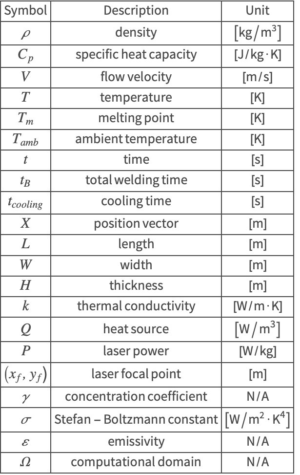
The symbols and corresponding units used here are summarized in the Nomenclature section.

Please refer to the information provided in "Heat Transfer" for a more general theoretical background for heat transfer analysis.

Load the finite element package.

Heat Transfer Model

The heat equation (1) is used to solve for the temperature field in a heat transfer model:

When modeling the heat transfer in a solid medium, there is no internal fluid flow that could cause a heat convection. Therefore the velocity term vanishes and the heat equation simplifies to

Since the internal convection introduced by the small amount of the melted steel is much weaker compared to the heat conduction that effect will be neglected in this model.

Set up the heat transfer model and material parameters for steel.

Set up material values.

Domain

Two steel pieces will be welded together will form a larger plate with a length of , a width of and the thickness of .

Specify the parameters of the geometry.

Define the 3D domain

In order to get a good result, a finer than the default grid is used for the mesh generation. Here we set the max edge length to be , which means that there will be at least one hundred elements in the (length) and (width) directions.

Discretize the domain with a prescribed mesh size.

Heat Source

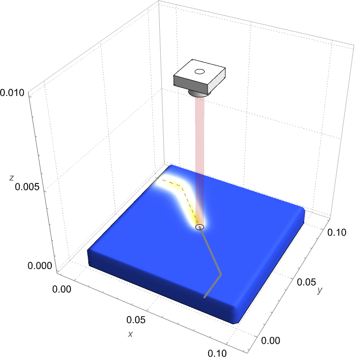
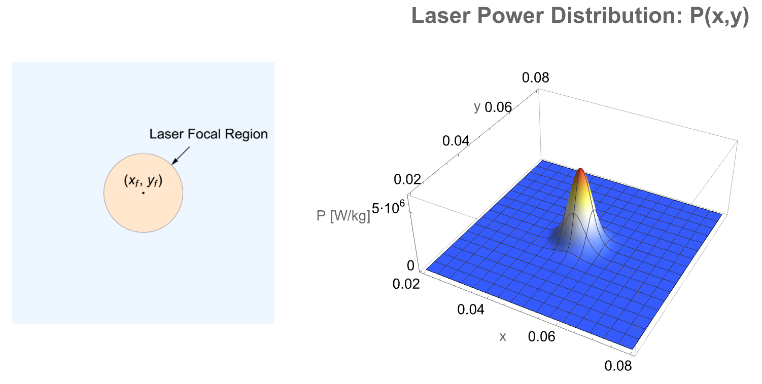
In this model the laser beam provides the thermal energy to weld the steel pieces, and is modeled by the heat source term in the heat equation (2). When applying the laser beam all particles within the focal region are irradiated and heated up simultaneously.

Assume the distribution of the laser power is described by a Gaussian bell shape at a focus point , and is homogeneous in the (thickness) direction. A parameter is introduced to control the degree of the laser concentration. A higher number implies a more concentrated beam.

The laser beam is applied for a total time of . The path of the beam follows the edges to be welded, and is describe as a function of time :

Define the path of the laser.

Set up the heat source term

for the laser beam with a laser power

and a concentration coefficient

Note, that all parameters except the independent variables are evaluated.

Initial and Boundary Conditions

At the beginning of the simulation, the temperature of the steel plate is assumed to be at the ambient temperature .

Set up the initial plate temperature

All the objects' surfaces are losing heat by radiation to the surrounding area. The Stefan-Boltzmann constant and the emissivity of steel are given by and , respectively.

Set up the thermal radiation boundary condition with HeatRadiationValue.

Solve the PDE Model

Next we will solve the heat transfer PDE model with NDSolve.

Set up the heat transfer PDE to be solved.

Define the simulation end time and solve the heat transfer model.

Post-processing and Visualization

To inspect the effect of the laser welding, we visualize the temperature distribution evolving in time.

Set up a legend bar and ContourPlot options for the temperature field plot.

Visualize the temperature field of the steel plate.

See this note about improving the visual quality of the animation.

Next, the maximum temperature is retrieved at each time step and compared with the melting point . Note that an effective welding requires during the welding process .

Extract the maximum temperature

at each time step.

Visualize the time profile of

Find the time

at which the plate temperature drops below the melting point

During the welding process: , the maximum temperature arises and exceeds the melting point , which confirms the effectiveness of the laser welding. For the joined steel plate gradually cools down by radiating to the surrounding, and drops below the melting point at .

Nomenclature

References

1. Abali B.E. Computational Reality: Solving Nonlinear and Coupled Problems in Continuum Mechanics. Advanced Structured Materials, vol 55. Springer, Singapore. (2017).

Top