Microscale Simulation of Catalyst Deactivation
| Introduction | Solve the PDE Model |
| Mass Transport Model | Appendix |
| Domain | Nomenclature |
| Material Parameters | References |
| Initial and Boundary Conditions |
Introduction
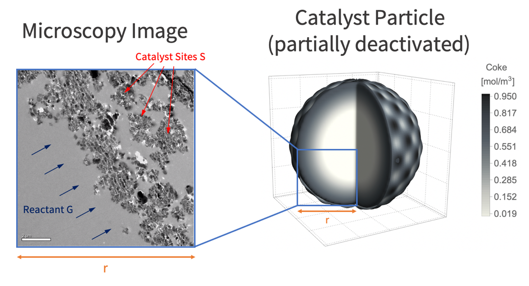
A catalyst is a substance that increases the rate of a chemical reaction without being consumed itself. Although it is not consumed, the catalyst can be deactivated by secondary processes. Two types of catalyst deactivation are common. First, the loss of a catalyst's reactivity, the ability to increase the rate of a reaction. Second, the loss of selectivity, the ability to direct a reaction to yield a particular product over time [1]. To avoid insufficient catalyst activity and selectivity, the deactivation of catalysts should be understood and monitored. This study is to simulate a gas-solid catalyst reaction within a porous structure and model the deactivation process over time.
The type of catalyst deactivation looked at in this study is due to coke accumulation [2]. In this case, coke accumulates over catalyst sites, ![]() , and reduces the catalyst's reactivity. In this model, a gas-phase reactant,
, and reduces the catalyst's reactivity. In this model, a gas-phase reactant, ![]() , is passed over a porous structure of a catalyst particle and is converted into a gas-phase product,
, is passed over a porous structure of a catalyst particle and is converted into a gas-phase product, ![]() . This product will then react with the catalyst as the secondary process and form coke,
. This product will then react with the catalyst as the secondary process and form coke, ![]() , on the catalyst sites. This coke accumulation eventually deactivates catalyst sites and reduces the rate of the reaction possible at the sites.
, on the catalyst sites. This coke accumulation eventually deactivates catalyst sites and reduces the rate of the reaction possible at the sites.

![]() is the reactant,
is the reactant,![]() is the catalyst sites,
is the catalyst sites,![]() is the product,
is the product,![]() is the accumulated coke,
is the accumulated coke,![]() are the reaction rate constants.
are the reaction rate constants.
To build a realistic geometry that represents the porous feature of a catalyst microstructure, an actual microscopy image of a catalyst particle [3] is used.
The catalyst particle is roughly assumed to be spherical. As such, the reactant's concentration will decrease with radius ![]() . Because of symmetry, it is then sufficient to use a 2D cutout of the catalyst particle for the simulation.
. Because of symmetry, it is then sufficient to use a 2D cutout of the catalyst particle for the simulation.
In this model, assume that there is no external fluid flow involved, which means the reactant ![]() is transported by diffusion only; there is no convective mass transfer.
is transported by diffusion only; there is no convective mass transfer.
To measure the level of the catalyst deactivation, the amount of coke ![]() that accumulates on the catalyst sites
that accumulates on the catalyst sites ![]() is computed. The net increase in the coke concentration is computed by integrating over the porous structure of the catalyst particle.
is computed. The net increase in the coke concentration is computed by integrating over the porous structure of the catalyst particle.
Here, ![]() denotes the local concentration of coke
denotes the local concentration of coke ![]() and
and ![]() denotes the mean concentration of coke
denotes the mean concentration of coke ![]() .
.
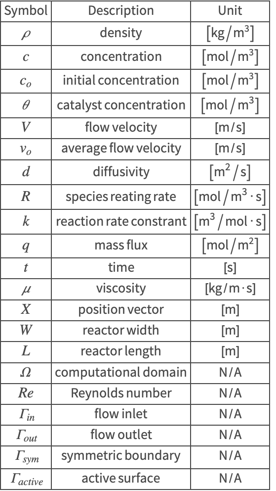
The symbols and corresponding units used here are summarized in the Nomenclature section.
Please refer to the information provided in the "Mass Transport" tutorial for a more general theoretical background for mass transport/chemical reaction analysis.
Needs["NDSolve`FEM`"]Mass Transport Model
The non-conservative mass transport equation (4) is used to solve for the concentration distribution ![]() in a mass transport model:
in a mass transport model:
![]() is the concentration of the transported species
is the concentration of the transported species ![]() ,
,![]() is the species diffusivity
is the species diffusivity ![]() ,
,![]() is the rate of mass production/consumption, the volumetric reacting rate of the species
is the rate of mass production/consumption, the volumetric reacting rate of the species ![]() .
.
The kinetic model of the catalyst reaction is given by:
Here, ![]() and
and ![]() are the reaction rate constants of this two-step process. First, the concentration evolution of reactant
are the reaction rate constants of this two-step process. First, the concentration evolution of reactant ![]() , catalyst sites
, catalyst sites ![]() and the resulting product
and the resulting product ![]() will be simulated. Once the concentration profile of
will be simulated. Once the concentration profile of ![]() ,
, ![]() and
and ![]() have been computed, the accumulation of coke
have been computed, the accumulation of coke ![]() based on the second step of the reaction in (5) can be determined.
based on the second step of the reaction in (5) can be determined.
During the first step, the concentration ![]() of the reactant
of the reactant ![]() denoted as
denoted as ![]() will reduce while the product concentration
will reduce while the product concentration ![]() increases. It is important to note that the concentration of catalyst sites
increases. It is important to note that the concentration of catalyst sites ![]() will only get consumed in the second reaction, resulting in a rise in the coke concentration
will only get consumed in the second reaction, resulting in a rise in the coke concentration ![]() .
.
Assume the catalyst reaction to be a first-order reaction [6]; that is, the reaction rate ![]() of each reacting species will be linearly proportional to the concentration of the involved reactants:
of each reacting species will be linearly proportional to the concentration of the involved reactants:
The values of rate constants ![]() and
and ![]() were estimated from the literature [7].
were estimated from the literature [7].
In this model, assume that there is no external fluid flow involved, which means the mass convection term: ![]() in (8) is set to zero and the mass is transported by diffusion only.
in (8) is set to zero and the mass is transported by diffusion only.
vars = {{Subscript[c, G][t, x, y], Subscript[c, S][t, x, y], Subscript[c, P][t, x, y]}, t, {x, y}};
MassTransportPDEComponent[vars, <|"DiffusionCoefficient" -> {{Subscript[d, G], 0, 0}, {0, Subscript[d, S], 0}, {0, Subscript[d, P], 0}}, "MassSource" -> {{-Subscript[k, 1] * Subscript[c, G][t, x, y] * Subscript[c, S][t, x, y]}, {-Subscript[k, 2] * Subscript[c, P][t, x, y] * Subscript[c, G][t, x, y]}, {(Subscript[k, 1] * Subscript[c, G][t, x, y] + Subscript[k, 2] * Subscript[c, P][t, x, y]) * Subscript[c, G][t, x, y]}}|>]
The reaction terms could very well also be modeled with a "MassReactionRate" model parameter in place of the "MassSource" term. Then a dependent variable needs to be factored out of the reaction rates and the sign of the equations negated. The choice is purely a matter of taste.
"MassReactionRate" -> {
	{0, Subscript[k, 1] * Subscript[c, G][t, x, y], 0},
	{0, Subscript[k, 2] * Subscript[c, P][t, x, y], 0},
	{0, -Subscript[k, 1] * Subscript[c, G][t, x, y] + Subscript[k, 2] * Subscript[c, P][t, x, y], 0}
};pars = <||>;k1 = 1 / 2;k2 = 3;
pars["MassSource"] = {
{-k1 * Subscript[c, G][t, x, y] * Subscript[c, S][t, x, y]},
{-k2 * Subscript[c, P][t, x, y] * Subscript[c, G][t, x, y]},
{(k1 * Subscript[c, G][t, x, y] + k2 * Subscript[c, P][t, x, y]) * Subscript[c, G][t, x, y]}
};Domain
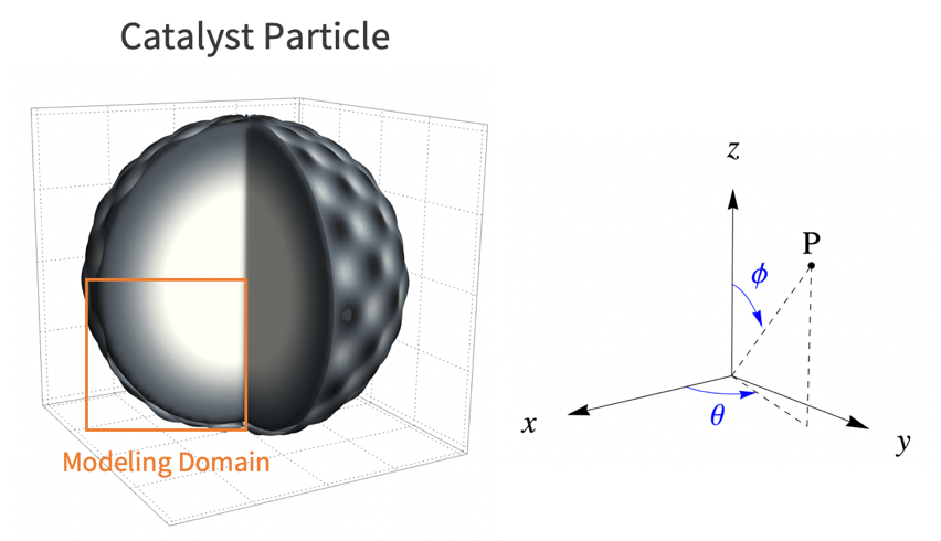
In this model, assume that the catalyst reaction occurs homogeneously from the particle surface into the core of the particle. As such, the variation of the species concentration in the azimuthal direction ![]() and the polar direction
and the polar direction ![]() can be ignored. Then a two dimensional model is sufficient to represent the 3D catalyst particle. Here the lower-left quarter of the catalyst particle is used as the modeling domain
can be ignored. Then a two dimensional model is sufficient to represent the 3D catalyst particle. Here the lower-left quarter of the catalyst particle is used as the modeling domain ![]() .
.
To build a realistic geometry that represents the catalyst microstructure, an actual microscopy image of the catalyst [9] is used. Note that the image needs to be binarized in order to distinguish the gas phase region (shown in white) and the solid phase region (shown in black).
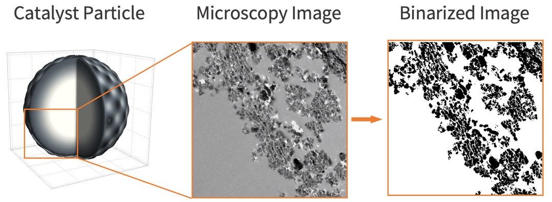
img = [image];binarizeImg = Binarize[img]The binarized image has a finely resolved catalyst boundary. When this image is discretized into a mesh, a large number of elements are expected. Since a large number of elements will result in a longer runtime and a larger memory usage, one may consider defeaturing the domain. Defeaturing is done by making use of a less accurate catalyst boundary, while still preserving the important characteristics of the original structure. The details about defeaturing the domain and its construction are presented in the appendix section: Construction of Defeatured Modeling Domain. For the sake of accuracy, the original region is used.
(*binarizeImg=DefeaturedBinarizeImg[img,5,100]*)Next, convert the binarized image into a mesh domain in order to apply the finite element method.
r = 12.36 * 10 ^ -6;
bmesh = ImageMesh[binarizeImg, Method -> "MarchingSquares"];
To model the catalyst reaction in a realistic scale, the domain is resized based on the radius of the catalyst particle measured in [10]: ![]() :
:
bmesh = RegionResize[bmesh, {{0, r}, {0, r}}];To generate the full element mesh, set up element markers to differentiate the gas phase region and the solid phase region. These markers can then be used to specify, for example, the species diffusivity![]() in different regions of the simulation domain.
in different regions of the simulation domain.
For markers to be attributed to different subregions, coordinates that lie in those subregions need to be specified. Here the coordinates of the solid phase region (catalyst sites ![]() ) are extracted.
) are extracted.
distTransform = DistanceTransform[ColorNegate[binarizeImg]];
maxima = MaxDetect[distTransform, 1];
components = ComponentMeasurements[{MorphologicalComponents[maxima], distTransform}, "Centroid"];
coordinates = components[[All, 2]] * r / ImageDimensions[img][[1]];
Show[bmesh, Graphics[{Red, Point[coordinates]}]]marker = {#, 1}& /@ coordinates;
mesh = ToElementMesh[bmesh, "RegionHoles" -> None, "RegionMarker" -> marker]
Rasterize[mesh["Wireframe"["MeshElementStyle" -> Map[...]]]]Here the gas-phase domain ![]() is shown in white and the solid-phase domain
is shown in white and the solid-phase domain ![]() is shown in blue. The two subregions are separated by internal mesh boundaries.
is shown in blue. The two subregions are separated by internal mesh boundaries.
More information on markers and their generation in meshes can be found in the Element Mesh Generation: Markers documentation.
Material Parameters
In this model, the diffusivity for the reactant ![]() and the product
and the product ![]() are different between the gas and solid domains. The diffusivity of the catalyst sites
are different between the gas and solid domains. The diffusivity of the catalyst sites ![]() is set to zero to represent its stationary feature:
is set to zero to represent its stationary feature:
Subscript[d, G] = Subscript[d, P] = If[ElementMarker == 1, 10^-13, 5 * 10^-11];
Subscript[d, S] = 0;
pars["DiffusionCoefficient"] = {{Subscript[d, G], 0, 0}, {0, Subscript[d, S], 0}, {0, 0, Subscript[d, P]}};
Also, see this note about how to set up computationally efficient PDE coefficients.
Initial and Boundary Conditions
In this model, the catalyst deactivating reaction is simulated for five seconds.
tend = 5;At ![]() , the initial concentrations for the reactant
, the initial concentrations for the reactant ![]() and the product
and the product ![]() are zero throughout the domain
are zero throughout the domain ![]() . The catalyst site
. The catalyst site ![]() is confined in the solid phase
is confined in the solid phase ![]() with an initial concentration of
with an initial concentration of ![]() .
.
A simple way to model the discontinuous initial concentration ![]() is by using the If statement with element markers:
is by using the If statement with element markers:
Subscript[c, S][0, x, y] == If[ElementMarker == 1, 1, 0];However, for the default second-order mesh, a discontinuous initial condition may result in overshoot/undershoot values for ![]() on the gas-solid interface due to the quadratic interpolation. This issue is explained in a separate tutorial: "Finite Element Method Usage Tips".
on the gas-solid interface due to the quadratic interpolation. This issue is explained in a separate tutorial: "Finite Element Method Usage Tips".
To improve the accuracy, use a linear interpolation instead. To do so, a first-order mesh is created and the original (second-order) interpolation result is extracted on first-order nodes. Then compute the linear interpolation based on these values.
meshFirstOrder = MeshOrderAlteration[mesh, 1];dof = Max[ElementIncidents[meshFirstOrder["MeshElements"]]];
resultSecondOrder = EvaluateOnElementMesh[{x, y}, If[ElementMarker == 1, 1, 0], mesh];
valuesOnNodes = Take[resultSecondOrder["ValuesOnGrid"], dof];CsLinear = ElementMeshInterpolation[{meshFirstOrder}, valuesOnNodes];ics =
{Subscript[c, G][0, x, y] == 0,
Subscript[c, S][0, x, y] == CsLinear[x, y],
Subscript[c, P][0, x, y] == 0};There are three types of boundary conditions involved in this mass transport model: the concentration boundary condition, the surrounding flux boundary condition, and the symmetric boundary condition.
The following illustration shows the locations where these boundary conditions are applied.
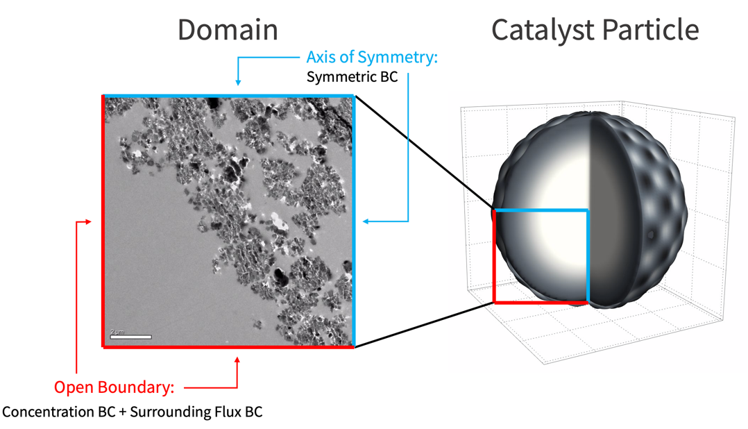
A default symmetric boundary condition is implicitly applied on the axis of symmetry.
A concentration boundary condition is used to model the supply of the reactant ![]() on the open surface. To avoid a discontinuous jump of reactant at the boundary, a helper function that smoothly ramps up the reactant supplied over time is created.
on the open surface. To avoid a discontinuous jump of reactant at the boundary, a helper function that smoothly ramps up the reactant supplied over time is created.
SmoothedStepFunction[fmin_, fmax_, ts_, m_] := Function[t, (fmin * Exp[ts * m] + fmax * Exp[m * t]) / (Exp[ts * m] + Exp[m * t])]GMin = 0;GMax = 2;ts = 1;m = 10;
GIn = SmoothedStepFunction[GMin, GMax, ts, m];
Plot[GIn[t], {t, 0, tend}, ...]Subscript[Γ, con] = MassConcentrationCondition[x == 0 || y == 0, {Subscript[c, G][t, x, y], t, {x, y}}, pars, <|"MassConcentration" -> {GIn[t]}|>]During the catalyst reaction, the product ![]() is free to diffuse out of the simulation domain through the open surface. This is modeled by a surrounding flux boundary condition.
is free to diffuse out of the simulation domain through the open surface. This is modeled by a surrounding flux boundary condition.
Subscript[Γ, flux] = MassTransferValue[x == 0 || y == 0, vars, pars, <|"MassTransferCoefficient" -> {0, 0, 10^-2}, "AmbientConcentration" -> 0|>]Solve the PDE Model
Concentration Field for G, S and P
First, the concentration field for the reactant ![]() , the catalyst sites
, the catalyst sites ![]() and the product
and the product ![]() is computed.
is computed.
pde = {MassTransportPDEComponent[vars, pars] == Subscript[Γ, flux], Subscript[Γ, con], ics};As mentioned in the previous section, due to the large number of elements, a longer runtime and a larger memory usage are expected than in typical application examples shown. The number of the degrees of freedom is proportional to the number of elements and gives a measure of the effort needed to solve a PDE.
Length[mesh["Coordinates"]]At each time step, three coupled PDEs need to be solved: ![]() (reactant
(reactant ![]() , product
, product ![]() and catalyst sites
and catalyst sites ![]() ) nodal values at each time step.
) nodal values at each time step.
3 * Length[mesh["Coordinates"]]Almost two million degrees of freedom need to be solved for.
measure = AbsoluteTiming[MaxMemoryUsed[Monitor[{GFun, SFun, PFun} = NDSolveValue[pde, {Subscript[c, G], Subscript[c, S], Subscript[c, P]}, {t, 0, tend}, {x, y}∈mesh, EvaluationMonitor :> (monitor = Row[{"t = ", CForm[t]}])], monitor]] / (1024. ^ 2)];
Print["Time -> ", measure[[1]], "
Memory -> ", measure[[2]]]boundaryHighlight = mesh["Wireframe"["MeshElement" -> "BoundaryElements"]];
GRange = MinMax[GFun["ValuesOnGrid"]];
SRange = MinMax[SFun["ValuesOnGrid"]];
PRange = MinMax[PFun["ValuesOnGrid"]];
GPlots = Rasterize[...]& /@ Append[...];
SPlots = Rasterize[...]& /@ Append[...];
PPlots = Rasterize[...]& /@ Append[...];
xlabels = {...};
ylabels = {...};
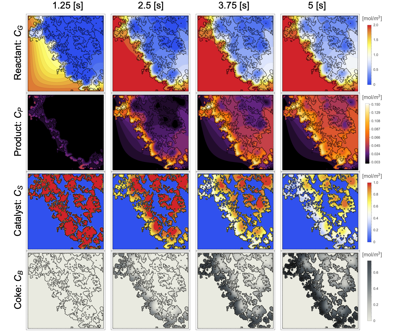
GraphicsGrid[...]During the reaction, the reactant ![]() gradually diffuses into the porous structure of the catalyst particle and is converted into the product
gradually diffuses into the porous structure of the catalyst particle and is converted into the product ![]() . This product
. This product ![]() then reacts within the porous structure and forms the coke
then reacts within the porous structure and forms the coke ![]() on the catalyst sites
on the catalyst sites ![]() . The coke accumulation eventually deactivates catalyst sites by decreasing the concentration of the catalyst sites.
. The coke accumulation eventually deactivates catalyst sites by decreasing the concentration of the catalyst sites.
The plots above are generated with a call to Rasterize. This is to reduce the disk space this notebook requires. To obtain high-quality graphics, comment out the call to Rasterize.
Concentration Field for B
Once the concentration field of the product ![]() and the catalyst
and the catalyst ![]() is computed, proceed to solve for the accumulation of coke
is computed, proceed to solve for the accumulation of coke ![]() based on the reaction equation:
based on the reaction equation:
The kinetic model for the accumulated coke ![]() is given by:
is given by:
To represent the stationary feature of the solid-phase coke ![]() , the diffusion coefficient is set to
, the diffusion coefficient is set to ![]() , and the equation (11) simplifies to:
, and the equation (11) simplifies to:
CokeModel = D[Subscript[c, B][t, x, y], {t, 1}] - k2 * PFun[t, x, y] * SFun[t, x, y];
pde = {CokeModel == 0, Subscript[c, B][0, x, y] == 0};measure = AbsoluteTiming[MaxMemoryUsed[Monitor[BFun = NDSolveValue[pde, Subscript[c, B], {t, 0, tend}, {x, y}∈mesh, EvaluationMonitor :> (monitor = Row[{"t = ", CForm[t]}])], monitor]] / (1024. ^ 2)];
Print["Time -> ", measure[[1]], "
Memory -> ", measure[[2]]]BRange = MinMax[BFun["ValuesOnGrid"]];
BPlots = Rasterize[...]& /@ Append[...];xlabels = {...};
ylabels = {Rotate[...]};
GraphicsGrid[...]The coke ![]() gradually accumulates throughout the porous structure of the catalyst particle over time. To measure the level of the coke accumulation, the increase in the mean coke concentration
gradually accumulates throughout the porous structure of the catalyst particle over time. To measure the level of the coke accumulation, the increase in the mean coke concentration ![]() is computed. This is done by integrating over the solid phase domain
is computed. This is done by integrating over the solid phase domain ![]() :
:
areaCatalyst =
	NIntegrate[Piecewise[{{1, ElementMarker == 1}, {0, True}}], {x, y}∈mesh];
Subscript[c, B, mean] = NIntegrate[BFun[tend, x, y], {x, y}∈mesh] / areaCatalyst
Due to the catalyst reaction, the coke ![]() has accumulated to
has accumulated to ![]() from
from ![]() to
to ![]() .
.
Appendix
Construction of Defeatured Modeling Domain
Due the large number of elements ![]() used, it took a significant amount of time/memory to solve this PDE model. To reduce the number of elements and the time/memory usage, the domain can be defeatured instead. That is, use a less accurate catalyst boundary but still preserve the important characteristics of the original structure.
used, it took a significant amount of time/memory to solve this PDE model. To reduce the number of elements and the time/memory usage, the domain can be defeatured instead. That is, use a less accurate catalyst boundary but still preserve the important characteristics of the original structure.
To build a defeatured domain, the catalyst boundary is smoothed out in the binarized image with DeleteSmallComponents.
DefeaturedBinarizeImg[image_, radius_, minimunPixelCount_] := DeleteSmallComponents[Opening[Binarize[image], DiskMatrix[radius]], minimunPixelCount]Here ![]() and
and ![]() are parameters that control the level of defeaturing and should be carefully chosen to preserve the accuracy of the modeling domain.
are parameters that control the level of defeaturing and should be carefully chosen to preserve the accuracy of the modeling domain.
g1 = Labeled[DefeaturedBinarizeImg[img, 5, 100], ...];
g2 = Labeled[binarizeImg, ...];
lis = Map[...];
GraphicsRow[...]
Note that the defeatured domain has a smoother catalyst boundary, which will significantly reduce the number of elements during the domain discretization.
defeaturedBmesh = ImageMesh[...];
defeaturedBmesh = RegionResize[defeaturedBmesh, {{0, r}, {0, r}}];
defeaturedMesh = ToElementMesh[defeaturedBmesh, "RegionHoles" -> None]meshNote that the mesh elements have been greatly reduced from 322k to 100k, leading to a lower time/memory consumption when solving the model.
The modeling result of the defeatured domain is given by:
Compared with the result from the original domain: here and here, it is seen that the catalyst reaction took a slightly longer time to propagate to the inner region through the porous structure. This is because some minor channels within the particle have been smoothed out and treated as a solid phase region with much smaller diffusivity, which makes it more difficult for the reactant ![]() to pass through.
to pass through.
Nomenclature
References
1. Bartholomew, C. H. "Mechanisms of Catalyst Deactivation," Applied Catalysis A: General, 212, pp. 17–60 (2001).
2. Wolf, E. E. and Alfani, F. "Catalysts Deactivation by Coking," Catalysis Reviews, vol 24, pp. 329–371 (1982).
3. Ciesielski, P. N., Robichaud, D., Donohoe, B. and Nimlos, M. "Microscale Simulation of Catalyst Deactivation during Gas-Phase Upgrading of Biomass Pyrolysis Vapors." Biosciences Center, National Renewable Energy Laboratory (2015).