Gas Absorption at Liquid Surface
| Introduction | Solve the PDE Model |
| Domain | Post-processing and Visualization |
| Mesh Generation | Nomenclature |
| Mass Transport Model | References |
| Boundary Conditions |
Introduction
Physical and chemical gas absorption are important separation processes and are widely employed in various industries. Gas absorption is used to either separate undesirable components from a gas or for manufacturing purposes of chemicals.
This example reproduces a gas absorption model [1]. The absorption process takes place in the gas-liquid interface section shown below in gray:
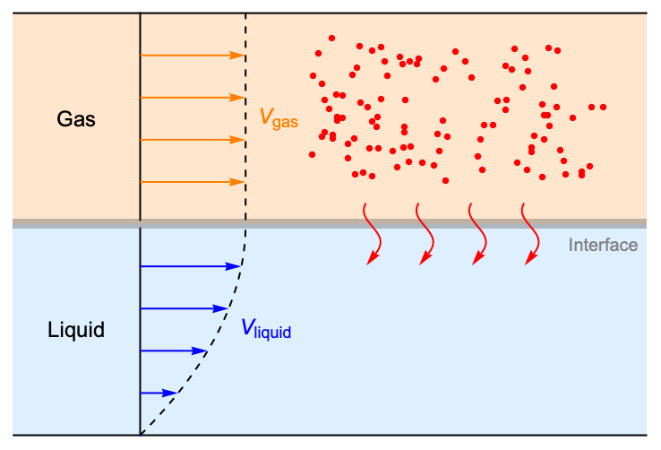
A gas is exposed to a fully developed laminar flow. The gas flows either cocurrently or countercurrently with respect to the flowing liquid. The above image displays the cocurrent case. The solute in the gas flow is absorbed and removed by the liquid flow beneath it, and mass transfer of the solute takes place from the gaseous to the liquid phase. The time of contact between solute and liquid is long enough to presume a parabolic velocity profile. Steady-state conditions are assumed to prevail. In the Post-processing section, the absorption effectiveness between the cocurrent case and the countercurrent case will be compared.
Needs["NDSolve`FEM`"]Domain
To model the interphase mass transfer, a thin interphase region is defined between the gas and liquid flow, which will allow an equilibrium condition (1) to be enforced, specified below via coupled fictitious mass sources, and to handle the discontinuous concentration of the solute between two different phases.
Here the thickness ![]() of the interphase region is set to be
of the interphase region is set to be ![]() of the height of the domain. Note that if
of the height of the domain. Note that if ![]() is set too small, numerical instability may occur around the interface.
is set too small, numerical instability may occur around the interface.
L = 1.5;
H1 = 0.5;
H2 = 0.5;
w = (H1 + H2) / 50;
Mesh Generation
Start by generating a boundary ElementMesh that accounts for the different material regions and the interface region. On the boundary, markers are specified that will be used later to set up boundary conditions for the cocurrent and countercurrent cases.
bmesh = ToBoundaryMesh["Coordinates" -> {...}, "BoundaryElements" -> {...}];
bmesh["Wireframe"["MeshElementMarkerStyle" -> Blue, "MeshElementStyle" -> {Orange, Red, Green, Black}]]boundary = <|"inletLeft" -> 1, "inletRight" -> 2, "inletLiquid" -> 3|>;To accurately model the mass transfer between the gas and liquid phases, the interphase region should be finely meshed. For clarity, the material regions are added as an Association.
material = <|"gas" -> 1, "interface" -> 2, "liquid" -> 3|>;
mesh = ToElementMesh[bmesh, "RegionMarker" -> {
	{{L / 2, H1 + H2 / 2}, material["gas"], 10^-3},
	{{L / 2, H1}, material["interface"], 10^-5},
{{L / 2, H1 / 2}, material["liquid"], 10^-3}}];mesh["Wireframe"["MeshElement" -> "MeshElements", "MeshElementStyle" -> {Directive[FaceForm[Orange]], Directive[FaceForm[Gray]], Directive[FaceForm[Blue]]}]]Mass Transport Model
A separate mass balance equation is used to describe the species concentration in the gas and liquid phases:
Here, ![]() and
and ![]() are the concentration of solute dissolved in the gas phase and liquid phase. To model the mass transfer between the two phases, coupling mass source terms
are the concentration of solute dissolved in the gas phase and liquid phase. To model the mass transfer between the two phases, coupling mass source terms ![]() and
and ![]() are added in the governing mass balance equation (2), leading to:
are added in the governing mass balance equation (2), leading to:
The above equations pose a system of two equations with both having three material regions.
vars = {{Subscript[c, gas][x, y], Subscript[c, liquid][x, y]}, {x, y}};
pars = <|"DiffusionCoefficient" -> {{Subscript[d, gas], 0}, {0, Subscript[d, liquid]}}, "MassConvectionVelocity" -> {{VectorSymbol[(Subscript[V, gas]), 2], 0}, {0, VectorSymbol[(Subscript[V, liquid]), 2]}}, "MassSource" -> {{Subscript[Q, gas]}, {Subscript[Q, liquid]}}|>;
MassTransportPDEComponent[vars, pars]
The diffusion coefficients of the solute in the gas and liquid phases are given by ![]() and
and ![]() , respectively. Note that
, respectively. Note that ![]() and
and ![]() are only active within the interphase region as well as their own phase.
are only active within the interphase region as well as their own phase.
pars[Subscript[d, gas]] = If[ElementMarker == material["gas"] || ElementMarker == material["interface"], 1, 0];
pars[Subscript[d, liquid]] = If[ElementMarker == material["liquid"] || ElementMarker == material["interface"], 0.1, 0];
Next, the fluid flow velocities ![]() are specified. The flow velocities are only active in their respective subregions. The gaseous flow velocity
are specified. The flow velocities are only active in their respective subregions. The gaseous flow velocity ![]() will initially be in the same direction as the liquid flow velocity
will initially be in the same direction as the liquid flow velocity ![]() .
.
pars[VectorSymbol[(Subscript[V, gas]), 2]] = {If[ElementMarker == material["gas"], 1, 0], 0};
pars[VectorSymbol[(Subscript[V, liquid]), 2]] = {If[ElementMarker == material["liquid"], Evaluate[(1 - ((y - H1) / H1) ^ 2), 0]], 0};
To model the mass transfer between two phases, the coupling mass source terms ![]() and
and ![]() are added in the governing mass balance equation (3), leading to:
are added in the governing mass balance equation (3), leading to:
Here, ![]() and
and ![]() are set at
are set at ![]() , so that the equilibrium condition (4)
, so that the equilibrium condition (4) ![]() can be enforced at the interface.
can be enforced at the interface.
In the equation, ![]() is the interphase mass transfer coefficient, and
is the interphase mass transfer coefficient, and ![]() is a switch that turns
is a switch that turns ![]() on within the interphase region and off
on within the interphase region and off ![]() otherwise.
otherwise.
pars[σ] = If[ElementMarker == material["interface"], 1, 0];Based on the two-resistance theory, the equilibrium at the interface is considered to be reached instantaneously and maintained at all times. This condition can be modeled by setting the mass transfer coefficient ![]() to be infinitely large. In practice,
to be infinitely large. In practice, ![]() can be chosen to be greater than the species diffusivity
can be chosen to be greater than the species diffusivity ![]() and
and ![]() ) by several orders of magnitude.
) by several orders of magnitude.
pars[k] = 10^4 * Max[(pars[Subscript[d, gas]] + pars[Subscript[d, liquid]]) /. {ElementMarker -> material["interface"]}]At the interface of two phases, the concentration ![]() and
and ![]() may be discontinuous. The ratio
may be discontinuous. The ratio ![]() is known as the equilibrium distribution coefficient
is known as the equilibrium distribution coefficient ![]() .
.
The coefficient ![]() depends on pressure, temperature and the chemical properties of the transported species and the media of both phases. The value
depends on pressure, temperature and the chemical properties of the transported species and the media of both phases. The value ![]() can be determined by experimental measurement [2]. In this example, the equilibrium coefficient is given by
can be determined by experimental measurement [2]. In this example, the equilibrium coefficient is given by ![]() .
.
pars[K] = 0.8;pars[Subscript[Q, gas]] = -pars[σ] * pars[k] * (pars[K] Subscript[c, gas][x, y] - Subscript[c, liquid][x, y]);
pars[Subscript[Q, liquid]] = -pars[Subscript[Q, gas]];Due to mass conservation, the coupling source terms ![]() and
and ![]() have the same magnitude but opposite sign.
have the same magnitude but opposite sign.
Also, see this note about how to set up computationally efficient PDE coefficients.
Boundary Conditions
The concentration of solute is set at ![]() at the gas inlet and
at the gas inlet and ![]() at the liquid inlet.
at the liquid inlet.
Subscript[Γ, gasIn] =
MassConcentrationCondition[ElementMarker == boundary["inletLeft"], vars, pars, <|"MassConcentration" -> {1, 0}|>]Subscript[Γ, liquidIn] =
MassConcentrationCondition[ElementMarker == boundary["inletLiquid"], vars, pars]Solve the PDE Model
pde = MassTransportPDEComponent[vars, pars] == {0, 0};{cFunGasCo, cFunliquidCo} = NDSolveValue[{pde, Subscript[Γ, gasIn], Subscript[Γ, liquidIn]}, {Subscript[c, gas], Subscript[c, liquid]}, {x, y}∈mesh];pars[VectorSymbol[(Subscript[V, gas]), 2]] = {If[ElementMarker == material["gas"], -1, 0], 0};
Subscript[Γ, gasIn] =
DirichletCondition[{Subscript[c, gas][x, y] == 1, Subscript[c, liquid][x, y] == 0}, ElementMarker == boundary["inletRight"]];
pdeModel = (MassTransportPDEComponent[vars, pars] == {0, 0});{cFunGasCounter, cFunliquidCounter} = NDSolveValue[{pdeModel, Subscript[Γ, gasIn], Subscript[Γ, liquidIn]}, {Subscript[c, gas], Subscript[c, liquid]}, {x, y}∈mesh];Post-processing and Visualization
legendBar = BarLegend[...];
Show[Legended[ContourPlot[cFunGasCo[x, y], ...], legendBar], ContourPlot[cFunliquidCo[x, y], ...], Graphics[...]]
To measure the effectiveness of the gas absorption, the net reduction of the solute is calculated between the gas inlet and outlet. For this, the mean concentration at the outlet is computed with a boundary integration:
Subscript[c, gasOut] = NIntegrate[cFunGasCo[L, y], {y, H1 + w / 2, H1 + H2}] / (H2 - w / 2)1 - Subscript[c, gasOut]In the cocurrent case, the solute in the gas flow has been reduced by ![]() .
.
Next, compare the result with the case of countercurrent gas and liquid flow.
Show[Legended[ContourPlot[cFunGasCounter[x, y], ...], legendBar], ContourPlot[cFunliquidCounter[x, y], ...], Graphics[...]]Subscript[c, gasOut] = NIntegrate[cFunGasCounter[0, y], {y, H1 + w / 2, H1 + H2}] / (H2 - w / 2)1 - Subscript[c, gasOut]In the countercurrent case, the solute in the gas flow has been reduced by ![]() , which is more effective than the cocurrent case.
, which is more effective than the cocurrent case.
Nomenclature
References
1. Danish, M., Sharma, R.K. and Ali, S. "Gas Absorption with First Order Chemical Reaction in a Laminar Falling Film over a Reacting Solid Wall," Applied Mathematical Modeling, 32, pp. 901–929 (2008).
2. Prausnitz, J. M., Lichtenthaler R. N. and de Azevedo, E. G. Molecular Thermodynamics of Fluid Phase Equilibria, 3rd ed., Prentice Hall PTR, New Jersey (1999).