Buoyancy-Driven Flow in a Square Cavity
| Introduction | Solve the PDE Model |
| Multiphysics Model | Post-processing and Visualization |
| Domain | Nomenclature |
| Boundary Conditions | References |
Introduction
Buoyancy-driven convection denotes a type of heat transfer in a fluid, in which the fluid flow is driven solely by a density difference due to a temperature gradient.
Consider a two-dimensional flow within a square cavity of solid walls, where gravity ![]() is acting in the
is acting in the ![]() direction. The left and right boundaries have different temperature values at
direction. The left and right boundaries have different temperature values at ![]() and
and ![]() , respectively. The top and bottom boundaries, however, are assumed to be thermally insulated.
, respectively. The top and bottom boundaries, however, are assumed to be thermally insulated.
As the fluid near the left boundary absorbs heat, it becomes less dense and rises due to thermal expansion. The surrounding cooler fluid then moves in to replace it, forming a convection current within the domain. This type of flow is known as natural/free convection.

The following simulation models the temperature, pressure and velocity fields within the square cavity. Since a stronger convection flow results in a higher rate of heat transfer, the level of the natural convection can be measured by calculating the heat flux ![]() at the boundary.
at the boundary.
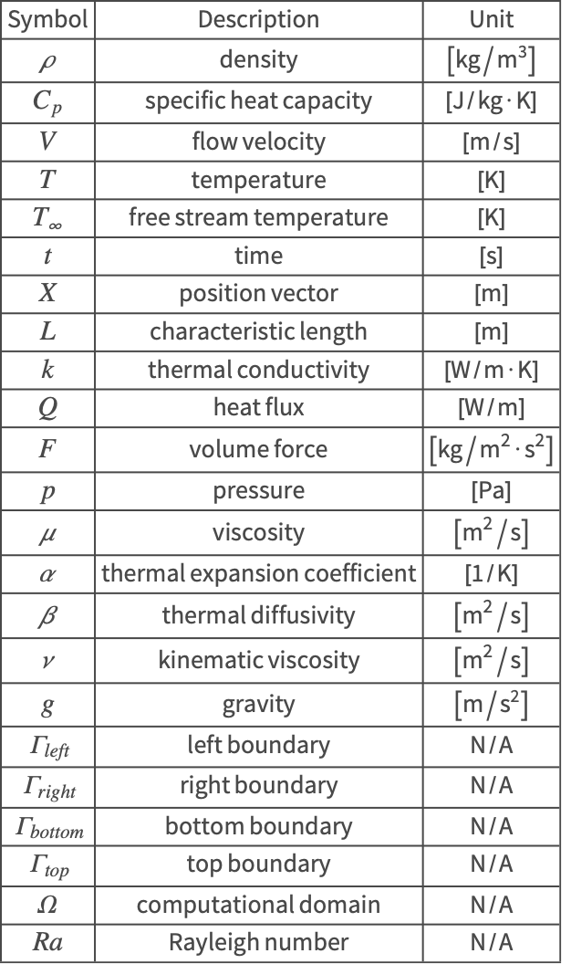
The symbols and corresponding units used here are summarized in the Nomenclature section.
Please refer to the information provided in "Heat Transfer" for a more general theoretical background for heat transfer analysis.
Needs["NDSolve`FEM`"]Multiphysics Model
Since this problem considers more than one kind of physics, a multiphysics model is constructed. The heat equation is coupled to the Navier–Stokes equation for modeling heat transfer with fluid flow.
Heat Transfer Model
For a steady-state heat transfer model without sources, the temperature distribution is described by the time-independent source-free heat equation (1). The heat convection by the fluid flow is modeled with the convective term. As such, the velocity field ![]() , specified through the fluid dynamics model, is set in the convective term
, specified through the fluid dynamics model, is set in the convective term ![]() of the heat equation:
of the heat equation:
varsT = {T[x, y], {x, y}};
parsT = <|"MassDensity" -> ρ, "SpecificHeatCapacity" -> Cp, "ThermalConductivity" -> k * IdentityMatrix[2], "HeatConvectionVelocity" -> {u[x, y], v[x, y]}|>;
SteadyHeatModel = HeatTransferPDEComponent[varsT, parsT]
Fluid Dynamics Model
The flow field is described by the steady-state Navier-Stokes equation (2). To account for the temperature effects on the fluid, a Boussinesq approximation [3] is used. This approximation neglects the variations in fluid properties except for the density differences induced by the temperature. In other words, the Boussinesq approximation assumes the buoyancy to be the only driving force acting on the fluid flow.
The buoyancy force appears in the source term ![]() in the Navier-Stokes equation:
in the Navier-Stokes equation:
varsCFD = {{u[x, y], v[x, y], p[x, y]}, {x, y}};
parsCFD = <|"MassDensity" -> ρ, "DynamicViscosity" -> μ|>;
CFDModel = FluidFlowPDEComponent[varsCFD, parsCFD]
Domain
The simulation domain ![]() is constructed as a unit square. The left, right, bottom and top boundaries are denoted by
is constructed as a unit square. The left, right, bottom and top boundaries are denoted by ![]() ,
, ![]() ,
, ![]() and
and ![]() , respectively:
, respectively:

Ω = Rectangle[];For a natural convection, the buoyancy is the driving force for the fluid motion. The fluid viscosity, on the other hand, is the dominant force that resisted this convection flow.
The dimensionless Rayleigh number ![]() [4] is then defined to represent the relationship between the buoyancy force and the viscosity force within the fluid:
[4] is then defined to represent the relationship between the buoyancy force and the viscosity force within the fluid:
![]() is the gravity
is the gravity ![]() ,
,![]() is the thermal expansion coefficient
is the thermal expansion coefficient ![]() ,
,![]() is the thermal diffusivity
is the thermal diffusivity ![]() ,
,![]() is the kinematic viscosity
is the kinematic viscosity ![]() ,
,![]() is the free stream temperature
is the free stream temperature ![]() .
.
In the following simulation, the convection flow field will be solved and compared under the Rayleigh numbers of ![]() and
and ![]() . The remaining flow properties are set as constants with a value of
. The remaining flow properties are set as constants with a value of ![]() .
.
parameters = {ρ -> 1, μ -> 1, Cp -> 1, k -> 1, Ra -> 10^3};Boundary Conditions
This multiphysics simulation contains both a heat transfer model and a fluid dynamics model and boundary conditions for each physics mode need to be set up.
Heat Transfer Model
There are two types of boundary conditions involved in the heat transfer model. At the left and right boundaries ![]() ,
, ![]() , the temperatures are held at
, the temperatures are held at ![]() and
and ![]() , respectively.
, respectively.
Subscript[Γ, temp] = {HeatTemperatureCondition[x == 0, varsT, parsT, <|"SurfaceTemperature" -> 1|>],
	HeatTemperatureCondition[x == 1, varsT, parsT, <|"SurfaceTemperature" -> 0|>]};
The top and bottom boundaries ![]() ,
, ![]() are assumed to be perfectly insulated. The default thermally insulated boundary conditions are implicitly applied.
are assumed to be perfectly insulated. The default thermally insulated boundary conditions are implicitly applied.
Fluid Dynamics Model
In the fluid dynamics model, the only boundary condition involved is the wall/no-slip boundary condition. At all four boundaries, the flow velocity ![]() is set to zero to model the solid walls where the fluid has no-slip.
is set to zero to model the solid walls where the fluid has no-slip.
Subscript[Γ, wall] = DirichletCondition[{u[x, y] == 0, v[x, y] == 0}, True];To solve for the flow pressure within the domain ![]() , a reference pressure is required. Here the reference point is chosen at the bottom-left point
, a reference pressure is required. Here the reference point is chosen at the bottom-left point ![]() with the reference pressure
with the reference pressure ![]() .
.
Subscript[Γ, p] = DirichletCondition[p[x, y] == 0, x == 0 && y == 0];bcs = {Subscript[Γ, temp], Subscript[Γ, wall], Subscript[Γ, p]};Solve the PDE Model
Recall that the Navier–Stokes equation is coupled to the heat equation by a Boussinesq approximation [5]. Since the buoyancy force is aligned with the ![]() axis, the source term in (6) is set up as
axis, the source term in (6) is set up as ![]() .
.
pde =
	{CFDModel == {0, Ra * T[x, y] * Cp * μ / k, 0}, SteadyHeatModel == 0, bcs} /. parameters;
A stable solution can be found if the velocities are interpolated with a higher order than the pressure. NDSolve allows an interpolation order for each dependent variable to be specified. Here the velocities ![]() and
and ![]() and the temperature
and the temperature ![]() are set to be interpolated with second order and the pressure
are set to be interpolated with second order and the pressure ![]() with first order.
with first order.
measure = AbsoluteTiming[MaxMemoryUsed[{ufun, vfun, pfun, Tfun} = NDSolveValue[pde, {u, v, p, T}, {x, y}∈Ω, Method -> {"PDEDiscretization" -> {"FiniteElement", "InterpolationOrder" -> {u -> 2, v -> 2, p -> 1, T -> 2}}}]] / (1024. ^ 2)];
Print["Time -> ", measure[[1]], "
Memory -> ", measure[[2]]]
Post-processing and Visualization
To inspect the heat transfer within the fluid flow, the following visualization combines the resulting velocity streamlines with the temperature distribution.
TRange = MinMax[Tfun["ValuesOnGrid"]];
legendBar = BarLegend[{"TemperatureMap", TRange}, ...];
options = {PlotRange -> TRange, ...};Show[Legended[ContourPlot[Tfun[x, y], ...], legendBar], VectorPlot[{ufun[x, y], vfun[x, y]}, ...]]To measure the amount of natural convection, the heat flux ![]() is calculated at the boundary
is calculated at the boundary ![]() . Note that a higher
. Note that a higher ![]() implies a stronger convection flow:
implies a stronger convection flow:
Because the top and bottom boundaries are thermally insulated, the heat flux ![]() across the left boundary
across the left boundary ![]() must equal the one across the right boundary
must equal the one across the right boundary ![]() , based on the energy conservation. Therefore, the heat flux
, based on the energy conservation. Therefore, the heat flux ![]() can be calculated at either
can be calculated at either ![]() or
or ![]() .
.
Q = Abs[NIntegrate[-k * Derivative[1, 0][Tfun][0, y] /. parameters, {y, 0, 1}]]In this case, the heat flux across the cavity is found as ![]() . This value matches the reference value
. This value matches the reference value ![]() presented in [7].
presented in [7].
Next, increase the Rayleigh number ![]() from
from ![]() to
to ![]() and solve for the convection flow field again.
and solve for the convection flow field again.
parameters = {ρ -> 1, μ -> 1, Cp -> 1, k -> 1, Ra -> 10^4};pde =
{CFDModel == {0, Ra * T[x, y] * Cp / μ, 0}, SteadyHeatModel == 0, bcs} /. parameters;To efficiently solve the updated heat transfer model, the previous result can be used as an initial guess for the new solution. Since the initial seeding based on the previous solution is already close to the final solution, the nonlinear solver will converge in fewer steps, resulting in less time elapsed.
measure = AbsoluteTiming[MaxMemoryUsed[{ufun2, vfun2, pfun2, Tfun2} = NDSolveValue[pde, {u, v, p, T}, {x, y}∈Ω, Method -> {"PDEDiscretization" -> {"FiniteElement", "InterpolationOrder" -> {u -> 2, v -> 2, p -> 1, T -> 2}}}, "InitialSeeding" -> {u[x, y] == ufun[x, y], v[x, y] == vfun[x, y], p[x, y] == pfun[x, y], T[x, y] == Tfun[x, y]}]] / (1024. ^ 2)];
Print["Time -> ", measure[[1]], "
Memory -> ", measure[[2]]]g1 = Show[...];
g2 = Show[...];
GraphicsRow[{g1, g2}, Spacings -> 0]When the Rayleigh number ![]() increases, the driving force (buoyancy) of the convective flow increases compared to the resisting force (viscosity) of the fluid motion. A stronger convection flow is then formed.
increases, the driving force (buoyancy) of the convective flow increases compared to the resisting force (viscosity) of the fluid motion. A stronger convection flow is then formed.
Q = Abs[NIntegrate[k * Derivative[1, 0][Tfun2][0, y] /. parameters, {y, 0, 1}]]The heat flux across the cavity has been increased from ![]() to
to ![]() , which implies a stronger convective heat transfer within the domain. This updated heat flux value also matches the reference value
, which implies a stronger convective heat transfer within the domain. This updated heat flux value also matches the reference value ![]() presented in [8].
presented in [8].
Nomenclature
References
1. D. de Vahl Davis and I. P. Jones. "Natural Convection of Air in a Square Cavity—A Comparison Exercise," International Journal for Numerical Methods in Fluids. Vol. 3 (1983).