Thermal Decomposition
| Introduction | Boundary Conditions |
| Multiphysics Model Setup | Solve the PDE Model |
| Physics Domains Coupling | Nomenclature |
| Domain | References |
| Flow Regime |
Introduction
Thermal decomposition is a chemical reaction where heat is a reactant. Since heat is a reactant, these reactions are endothermic, meaning that the reaction requires thermal energy to break the chemical bonds in the molecule. A classic example is the calcination process:
Calcium carbonate, ![]() , will decompose into carbon dioxide,
, will decompose into carbon dioxide, ![]() , and calcium oxide,
, and calcium oxide, ![]() , when heated above
, when heated above ![]() at a pressure of
at a pressure of ![]() atmosphere. For endothermic reactions, in this case the heat of reaction,
atmosphere. For endothermic reactions, in this case the heat of reaction, ![]() , is negative. This reaction is known as the common way to make quicklime,
, is negative. This reaction is known as the common way to make quicklime, ![]() , which is an industrially important product.
, which is an industrially important product.
This study is to model the decomposition process of calcium carbonate and simulate its concentration field within an expanding reactor. The calcium carbonate is transported into the reactor by suspending it in water that enters the domain from the bottom, flows across a heated tube and exits the reactor through the top. During this process, the calcium carbonate particles decompose and absorb heat from the system.
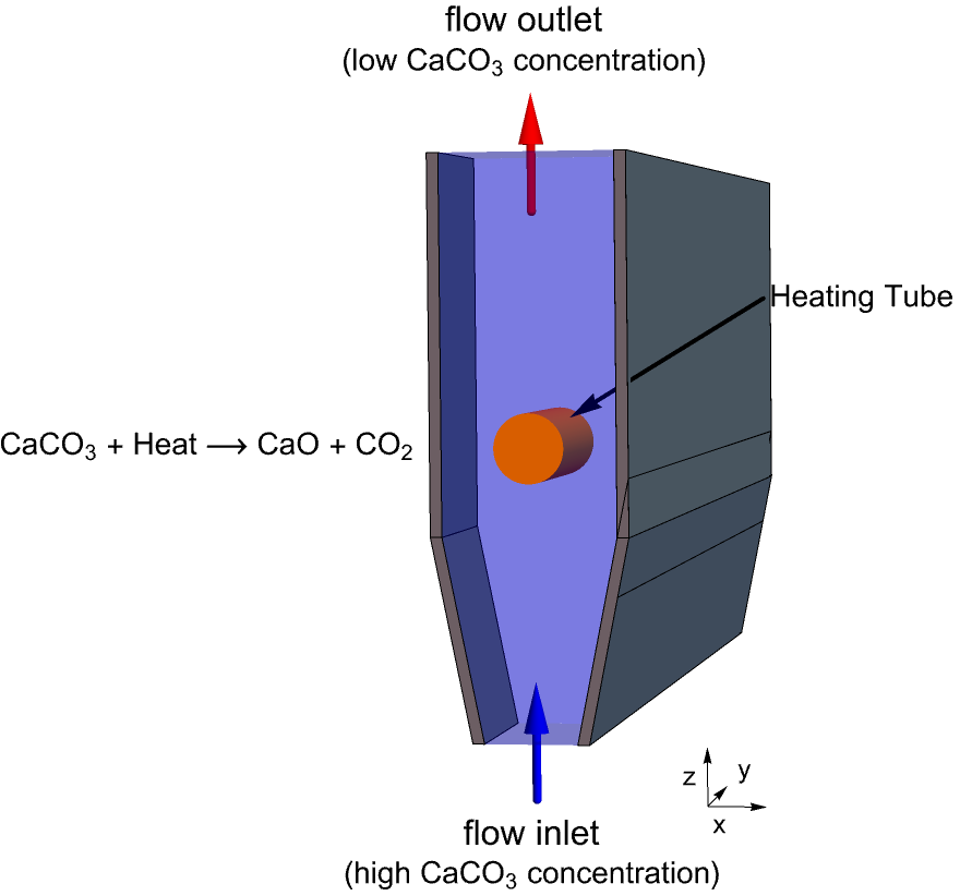
Calculating net reduction in the ![]() concentration between the flow inlet
concentration between the flow inlet ![]() and outlet
and outlet ![]()
![]() can be used to express the effectiveness of the reactor.
can be used to express the effectiveness of the reactor.
The mean ![]() concentration at a boundary
concentration at a boundary ![]() is computed from the integral:
is computed from the integral:
using NIntegrate.
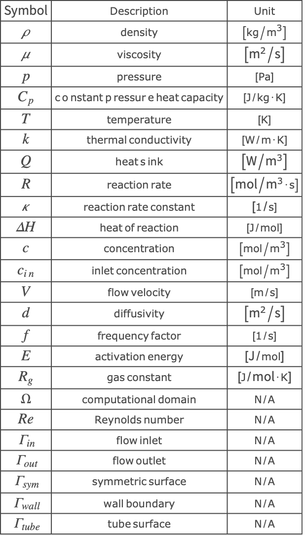
The symbols and corresponding units used for this model are summarized in the Nomenclature section.
Please refer to the information provided in the Heat Transfer Tutorial and Mass Transport Tutorial for a more general theoretical background for this multiphysics model.
Needs["NDSolve`FEM`"]Multiphysics Model Setup
Since this problem considers more than one physics domain, a multiphysics model is to be constructed. As a first step, the contributing physics domains are looked at independently. A fluid dynamics model, a heat transfer model and a mass transport model are set up to solve for the flow field ![]() , temperature field
, temperature field ![]() and concentration field
and concentration field ![]() within the reactor.
within the reactor.
Fluid Dynamics Model
The Navier–Stokes equation (1) is used to solve for the steady–state flow field ![]() within the reactor. Note that a 2D domain
within the reactor. Note that a 2D domain ![]() is used to simulate the 3D reactor. The reason for this model order reduction will be explain in the later section about the modeling domain setup.
is used to simulate the 3D reactor. The reason for this model order reduction will be explain in the later section about the modeling domain setup.
![]() is the density
is the density ![]() ,
,![]() is the viscosity
is the viscosity ![]() ,
,![]() is the velocity field
is the velocity field ![]() ,
,![]() is the pressure
is the pressure ![]() .
.
CFDModel =
	{ρ {u[x, y], v[x, y]}.Inactive[Grad][u[x, y], {x, y}] + Inactive[Div][(-μ)*Inactive[Grad][u[x, y], {x, y}], {x, y}] + p^(1, 0)[x, y],
	ρ {u[x, y], v[x, y]}.Inactive[Grad][v[x, y], {x, y}] + Inactive[Div][(-μ)*Inactive[Grad][v[x, y], {x, y}], {x, y}] + p^(0, 1)[x, y], u^(1, 0)[x, y] + v^(0, 1)[x, y]};
Heat Transfer Model
For a steady-state heat transfer model, the temperature distribution ![]() is described by the steady-state heat equation (2). The heat convected by the fluid flow is modeled with the convective term:
is described by the steady-state heat equation (2). The heat convected by the fluid flow is modeled with the convective term: ![]() .
.
Since the thermal decomposition is an endothermic process, the heat absorbed by the reaction is modeled by the heat sink term ![]() , which depends on both the chemical reaction rate,
, which depends on both the chemical reaction rate, ![]() , and the heat of reaction,
, and the heat of reaction, ![]() :
:
![]() is the constant pressure heat capacity
is the constant pressure heat capacity ![]() ,
,![]() is the temperature
is the temperature ![]() ,
,![]() is the thermal conductivity
is the thermal conductivity ![]() ,
,![]() is the heat sink
is the heat sink ![]() ,
,![]() is the reaction rate
is the reaction rate ![]() ,
,![]() is the heat of reaction
is the heat of reaction ![]() .
.
tvars = {T[x, y], {x, y}};
SteadyHeatModel = HeatTransferPDEComponent[tvars, <|"MassDensity" -> ρ, "SpecificHeatCapacity" -> Cp, "ThermalConductivity" -> k * IdentityMatrix[2], "HeatConvectionVelocity" -> {u[x, y], v[x, y]}, "HeatSource" -> Q|>]
Mass Transport Model
The steady-state mass transport equation (3) is used to solve for the concentration field ![]() within the reactor. The mass transported by the flow field is modeled by the convective term
within the reactor. The mass transported by the flow field is modeled by the convective term ![]() .
.
The chemical reaction rate ![]() depends on both the reactant concentration
depends on both the reactant concentration ![]() and the reaction rate constant
and the reaction rate constant ![]() .
.
Note that for decomposition reactions, the reaction rate, ![]() , is negative.
, is negative.
The rate constant ![]() is temperature dependent according to the Arrhenius equation [4]:
is temperature dependent according to the Arrhenius equation [4]:
Note that the standard notation of the reaction constant is denoted by ![]() ; however, to avoid the conflict with thermal conductivity in this case, the nonstandard symbol
; however, to avoid the conflict with thermal conductivity in this case, the nonstandard symbol ![]() is used instead.
is used instead.
![]() is the concentration of
is the concentration of ![]()
![]() ,
,![]() is the species diffusivity
is the species diffusivity ![]() ,
,![]() is the frequency factor
is the frequency factor ![]() ,
,![]() is the activation energy
is the activation energy ![]() ,
,![]() is the gas constant
is the gas constant ![]() .
.
Even though the gas constant ![]() is involved in (5), the Arrhenius equation is not limited to gas-phase reactions.
is involved in (5), the Arrhenius equation is not limited to gas-phase reactions.
cvars = {c[x, y], {x, y}};
SteadyMassModel = MassTransportPDEComponent[cvars, <|"DiffusionCoefficient" -> d * IdentityMatrix[2], "MassSource" -> R, "MassConvectionVelocity" -> {u[x, y], v[x, y]}|>]
Physics Domains Coupling
Once all the contributing physics domains are set up, the type of coupling involved in order to simulate the interaction between the different physical phenomena needs to be investigated.
As described in the previous section, the temperature field ![]() within the reactor is computed with the heat equation (6) and depends on both the fluid flow velocity
within the reactor is computed with the heat equation (6) and depends on both the fluid flow velocity ![]() computed with the Navier–Stokes equation (7) and the concentration
computed with the Navier–Stokes equation (7) and the concentration ![]() through reaction rate
through reaction rate ![]() of the mass transport equation (8). Furthermore, the reaction rate
of the mass transport equation (8). Furthermore, the reaction rate ![]() itself also depends on the temperature
itself also depends on the temperature ![]() from the heat equation (9), resulting in a nonlinear, two-way relation between each physical mode.
from the heat equation (9), resulting in a nonlinear, two-way relation between each physical mode.
To solve a two-way coupled nonlinear PDE system like this, a possible strategy is to first solve a simpler model with a weaker nonlinearity and use the solution of the simpler model as an initial guess for the full nonlinear model. Ignoring the heat generated by the reaction gives a good simpler model to start with. This approach is detailed in the following sections.
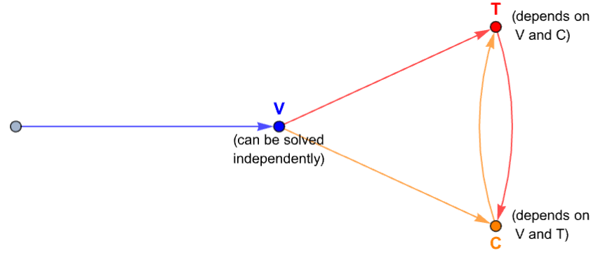
One-Way Coupled Multiphysics Model
By ignoring the heat of reaction (i.e. ![]() ,
, ![]() ) from the decomposition, the heat equation (10) is simplified to
) from the decomposition, the heat equation (10) is simplified to ![]() . This leads to an one-way coupled multiphysics model. For clarity, the dependent variable for each physical mode is highlighted:
. This leads to an one-way coupled multiphysics model. For clarity, the dependent variable for each physical mode is highlighted:
The dependency of the one-way coupled model can be illustrated as:
This one-way coupled multiphysics model can either be solved sequentially or in one go. Solving it sequentially would mean that each of the physics domains is solved with a separate call to NDSolve. This approach of splitting the coupled equations in chunks and solving them independently and sequentially is called a segregated solution process. In case the single physics fields cannot be split easily, an initial guess for the coupling variable of the first PDE is made. Then the solution of the first PDE is taken to drive the next PDE and so forth. Once all PDEs have been solved, the process is started over again. This will improve the initial guess for the initial coupling variable. This procedure is executed until the solution converges.
Fully Coupled Multiphysics Model
Once the one-way coupled model is solved, the solution can be used as an initial guess for the fully nonlinear model. Here the fully coupled model is built by adding the heat of reaction ![]() .
.

The dependency of the fully coupled model can be illustrated as:
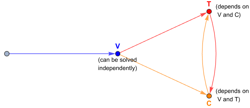
Note that the temperature field ![]() and the concentration field
and the concentration field ![]() would affect each other and should therefore be solved as a system of PDEs in NDSolve. This solving process will be shown in the later section Solve the PDE Model: Fully Coupled Model Solution.
would affect each other and should therefore be solved as a system of PDEs in NDSolve. This solving process will be shown in the later section Solve the PDE Model: Fully Coupled Model Solution.
Material Parameters
To solve any of the proposed multiphysics models, material properties need to be specified for both the fluid medium and the calcium carbonate ![]() .
.
Subscript[ρ, water] = QuantityMagnitude[ThermodynamicData["Water", "Density"]];
Subscript[k, water] = QuantityMagnitude[ThermodynamicData["Water", "ThermalConductivity"]];
Subscript[μ, water] = QuantityMagnitude[ThermodynamicData["Water", "Viscosity"]];
Subscript[Cp, water] = QuantityMagnitude[ThermodynamicData["Water", "IsobaricHeatCapacity"]];Subscript[d, Subscript[CaCO, 3]] = 2 * 10^-9;
Subscript[e, Subscript[CaCO, 3]] = 304.6 * 10^3;
Subscript[f, Subscript[CaCO, 3]] = 4.67 * 10^14;
Subscript[H, Subscript[CaCO, 3]] = -178 * 10^3;Note that the heat of reaction ![]() , which means the reaction is endothermic.
, which means the reaction is endothermic.
Subscript[R, g] = N[First[UnitConvert[Quantity["MolarGasConstant"]]]];parameters = {ρ -> Subscript[ρ, water], k -> Subscript[k, water], μ -> Subscript[μ, water], Cp -> Subscript[Cp, water], d -> Subscript[d, Subscript[CaCO, 3]]};Domain
The expanding reactor model is bounded by two symmetric plates as shown below:

Since the depth (![]() direction) of the reactor is considerably more than its width (
direction) of the reactor is considerably more than its width (![]() direction) and its height (
direction) and its height (![]() direction), it is reasonable to neglect the variation of
direction), it is reasonable to neglect the variation of ![]() in the
in the ![]() direction, so a two-dimensional model is sufficient to represent the 3D reactor:
direction, so a two-dimensional model is sufficient to represent the 3D reactor:

As a further step to simplify the geometry, note the symmetry about the vertical (![]() ) axis. It is effective to only make use of the right half of the reactor as the simulation domain
) axis. It is effective to only make use of the right half of the reactor as the simulation domain ![]() . Here
. Here ![]() and
and ![]() denote the flow inlet and flow outlet. The wall boundary and the symmetric axis are symbolized as
denote the flow inlet and flow outlet. The wall boundary and the symmetric axis are symbolized as ![]() and
and ![]() , respectively.
, respectively.
For the sake of simplicity, ![]() is used to denote the 2D domain
is used to denote the 2D domain ![]() in the following sections.
in the following sections.
W1 = 8 * 10^-3;
W2 = 15 * 10^-3;
H1 = 35 * 10^-3;
H2 = 100 * 10^-3;
r = 6 * 10^-3;
Subscript[x, tube] = 0;
Subscript[y, tube] = 50 * 10^-3;Ω = RegionDifference[Rectangle[{0, 0}, {W2, H2}], RegionUnion[Disk[{Subscript[x, tube], Subscript[y, tube]}, r], Triangle[{{W1, 0}, {W2, H1}, {W2, 0}}]]];In order to get a good result, a grid finer than the default is used for the mesh generation. Here, the maximum grid size is set to ![]() , which means that there will be about a hundred elements in the
, which means that there will be about a hundred elements in the ![]() direction (height).
direction (height).
mesh = ToElementMesh[Ω, "MaxCellMeasure" -> {"Length" -> 10 ^ -3}]Flow Regime
When a simulation involves fluid flow, it is advisable to calculate the Reynolds number to determine the type of the flow. Empirically, the flow is considered as laminar when ![]() and as turbulent when
and as turbulent when ![]() . For a Reynolds number between roughly
. For a Reynolds number between roughly ![]() , an unsteady separation of flow may form around blunt bodies [11], resulting in an oscillating vortex shedding in the flow field. Whenever this happens, the steady-state fluid dynamics model will fail to converge, and a steady-state solution is not achievable.
, an unsteady separation of flow may form around blunt bodies [11], resulting in an oscillating vortex shedding in the flow field. Whenever this happens, the steady-state fluid dynamics model will fail to converge, and a steady-state solution is not achievable.
The Reynolds number for a flow is calculated as:
In this model, the incoming flow has an average velocity of ![]() , and the characteristic length is taken as the diameter of the heating wire:
, and the characteristic length is taken as the diameter of the heating wire: ![]() .
.
"Re" -> (ρ v L/μ) /. {v -> 5 * 10^-4, L -> 1.2 * 10^-2, ρ -> Subscript[ρ, water], μ -> Subscript[μ, water]}The parameters for the reactor are chosen so that the Reynolds number falls into the laminar flow regime, which means the chemical reactor in this case is a laminar flow reactor (LFR). One feature of the LFR is the higher residence time [12] (the time interval during which the chemicals stay in the reactor), and this is desirable for the calcination to achieve a higher production rate.
Boundary Conditions
This multiphysics simulation contains both a heat transfer model and a fluid dynamics model and boundary conditions for each physics mode need to be set up.
Note that the boundary conditions used in both solution approaches (one-way coupling versus full coupling) are the same.
Fluid Dynamics Boundary Conditions
There are four types of boundary conditions involved in the fluid dynamics model. At the inlet, the flow velocity is set to ![]() .
.
Subscript[v, in] = 5 * 10^-4;
Subscript[Γ, vel] = DirichletCondition[{u[x, y] == 0, v[x, y] == Subscript[v, in]}, y == 0];
On the walls of the reactor, the flow velocity is set to zero to model a no-slip flow condition.
Subscript[Γ, wall] = DirichletCondition[{u[x, y] == 0, v[x, y] == 0}, x > 0 && 0 < y < H2];Due to the symmetry along the ![]() axis, the velocity in the
axis, the velocity in the ![]() direction is set to zero at the symmetry boundaries
direction is set to zero at the symmetry boundaries ![]() .
.
Subscript[Γ, sym] = DirichletCondition[u[x, y] == 0, x == 0];At the top boundary, a pressure outlet boundary condition is used to model the outgoing flow. Here, the outlet pressure is set equal to the ambient pressure ![]() .
.
Subscript[Γ, outlet] = DirichletCondition[p[x, y] == 0, y == H2];Heat Transfer Boundary Conditions
There are four types of boundary conditions involved in the heat transfer model. At the flow inlet ![]() and the tube surface
and the tube surface ![]() , the temperatures are set to
, the temperatures are set to ![]() and
and ![]() , respectively.
, respectively.
Subscript[T, in] = 950;Subscript[T, tube] = 975;
Subscript[Γ, temp] = {HeatTemperatureCondition[y == 0, tvars, <||>, <|"SurfaceTemperature" -> Subscript[T, in]|>], HeatTemperatureCondition[(x - Subscript[x, tube])^2 + (y - Subscript[y, tube])^2 ≤ (r + 10 * $MachineEpsilon)^2, tvars, <||>, <|"SurfaceTemperature" -> Subscript[T, tube]|>]}
The wall boundaries are assumed to be perfectly thermally insulated and are modeled by a thermally insulated boundary condition. An outflow boundary condition and a symmetric boundary condition are applied on the flow outlet ![]() and the symmetric axis
and the symmetric axis ![]() , respectively.
, respectively.
However, since the outflow boundary condition, symmetric boundary condition and thermally insulated boundary condition are all Neumann zero conditions, they are implicitly applied without further setup.
Mass Transport Boundary Conditions
There are four types of boundary conditions involved in the mass transfer model. Assuming an infinite supply of the species, the concentration at the flow inlet ![]() is then held at
is then held at ![]() .
.
Subscript[c, in] = 10^3;
Subscript[Γ, con] = MassConcentrationCondition[y == 0, cvars, <||>, <|"MassConcentration" -> Subscript[c, in]|>]
On the walls of the reactor, the mass flux of the species is assumed to be zero and is modeled by an impermeable boundary condition. An outflow boundary condition and a symmetric boundary condition are applied on the flow outlet ![]() and the symmetric axis
and the symmetric axis ![]() , respectively.
, respectively.
However, since the impermeable boundary condition, outflow boundary condition and symmetric boundary condition are all Neumann zero conditions, they are implicitly applied without further setup.
Solve the PDE Model
One-Way Coupled Model Solution
In the following section, the one-way coupled multiphysics model will be solved sequentially for each physics mode.
Fluid dynamics model
First, the fluid dynamics PDE is solved for the flow velocity field ![]() .
.
pde = {CFDModel == {0, 0, 0}, Subscript[Γ, vel], Subscript[Γ, outlet], Subscript[Γ, wall], Subscript[Γ, sym]} /. parameters;A stable solution can be found if the velocities are interpolated with a higher order than the pressure. NDSolve allows an interpolation order for each dependent variable to be specified. Here, the velocities ![]() and
and ![]() are set to be interpolated with second order and the pressure
are set to be interpolated with second order and the pressure ![]() with first order.
with first order.
{uFun, vFun, pressureFun} = NDSolveValue[pde, {u, v, p}, {x, y}∈mesh, Method -> {"PDEDiscretization" -> {"FiniteElement", "InterpolationOrder" -> {u -> 2, v -> 2, p -> 1}}}];To inspect the fluid field within the reactor, the following visualization combines a vector plot for velocity streamlines where ![]() and a contour plot for the velocity magnitude with
and a contour plot for the velocity magnitude with ![]() .
.
boundaryHighlight = Graphics[{...}];
VRange = MinMax[vFun["ValuesOnGrid"]];
Show[Legended[ContourPlot[Sqrt[uFun[x, y]^2 + vFun[x, y]^2], ...], BarLegend[...]], VectorPlot[{uFun[x, y], vFun[x, y]}, {x, y}∈Ω, ...], boundaryHighlight]MinMax[uFun["ValuesOnGrid"]]MinMax[vFun["ValuesOnGrid"]]It is seen that the flow velocity ![]() decreases along the expansion region and increases around the tube.
decreases along the expansion region and increases around the tube.
Heat transfer model
With the flow field ![]() in hand, the heat transfer model can be solved for the steady-state temperature field
in hand, the heat transfer model can be solved for the steady-state temperature field ![]() .
.
pde = {SteadyHeatModel == 0, Subscript[Γ, temp]} /. parameters /. {u -> uFun, v -> vFun, Q -> 0};
temperatureFun = NDSolveValue[pde, T, {x, y}∈mesh];MinMax[temperatureFun["ValuesOnGrid"]]tempPlotRange = {925, 975};Show[Legended[ContourPlot[temperatureFun[x, y], {x, y}∈mesh, ...], BarLegend[...]], boundaryHighlight]The flow enters the reactor at a temperature of ![]() and is heated as it passes by the heating tube
and is heated as it passes by the heating tube ![]() . Note that since reaction heat generated is ignored in this case, the temperature variance is caused by the tube heating only.
. Note that since reaction heat generated is ignored in this case, the temperature variance is caused by the tube heating only.
Next the concentration field ![]() of the species will be solved for.
of the species will be solved for.
Mass transport model
As described in the previous section, ![]() particles within the reactor are decomposing at a reaction rate
particles within the reactor are decomposing at a reaction rate ![]() .
.
Subscript[R, Subscript[CaCO, 3]] = -Subscript[f, Subscript[CaCO, 3]] * Exp[-Subscript[e, Subscript[CaCO, 3]] / (Subscript[R, g] * temperatureFun[x, y])] * c[x, y];pde = {SteadyMassModel == 0, Subscript[Γ, con]} /. parameters /. {u -> uFun, v -> vFun, R -> Subscript[R, Subscript[CaCO, 3]]};
concentrationFun = NDSolveValue[pde, c, {x, y}∈mesh];MinMax[concentrationFun["ValuesOnGrid"]]Show[Legended[ContourPlot[concentrationFun[x, y], ...], BarLegend[...]], boundaryHighlight]The concentration of ![]() is held at
is held at ![]() at the inlet and then deceases as it flows over the reactor due to decomposition. Note that the
at the inlet and then deceases as it flows over the reactor due to decomposition. Note that the ![]() concentration drops significantly in the lower part of the reactor because of the higher reaction rate. This can be verified by visualizing the reaction rate field:
concentration drops significantly in the lower part of the reactor because of the higher reaction rate. This can be verified by visualizing the reaction rate field: ![]() .
.
Show[Legended[
	ContourPlot[(Subscript[f, Subscript[CaCO, 3]] Exp[-(Subscript[e, Subscript[CaCO, 3]]/Subscript[R, g] * temperatureFun[x, y])]) concentrationFun[x, y], ...], BarLegend[...]], boundaryHighlight]
Note that a significant decomposition occurs in the lower part of the reactor around the flow inlet. This explains why the previous plot showed a significant drop of ![]() concentration in this region.
concentration in this region.
Fully Coupled Model Solution
Using the one-way coupling model, the flow velocity ![]() , temperature
, temperature ![]() and the
and the ![]() concentration
concentration ![]() have been solved for in a sequential manner. Now a fully coupled model is solved and the difference in solution investigated.
have been solved for in a sequential manner. Now a fully coupled model is solved and the difference in solution investigated.
The heat of reaction ![]() that was previously ignored will now be added. This leads to a nonlinear, fully coupled relation between the heat equation and the mass transport equation.
that was previously ignored will now be added. This leads to a nonlinear, fully coupled relation between the heat equation and the mass transport equation.
In the previous section, it has been shown that the heat source term ![]() depends the reaction rate
depends the reaction rate ![]() by:
by:
Subscript[R, Subscript[CaCO, 3]] = -Subscript[f, Subscript[CaCO, 3]] * Exp[-Subscript[e, Subscript[CaCO, 3]] / (Subscript[R, g] * T[x, y])] * c[x, y];
Subscript[Q, Subscript[CaCO, 3]] = -Subscript[H, Subscript[CaCO, 3]] * Subscript[R, Subscript[CaCO, 3]];CoupledMassModel = SteadyMassModel /. R -> Subscript[R, Subscript[CaCO, 3]];
CoupledHeatModel = SteadyHeatModel /. Q -> Subscript[Q, Subscript[CaCO, 3]];To efficiently solve the coupled PDE model, the result from the previous step is used as an initial seed for the new solution. In fact not doing so will result in a model where the nonlinear solver does not converge. It is a general strategy to first solve a less nonlinear model and use the solution thereof as an initial seed for a more nonlinear model.
pde = {CoupledMassModel == 0, CoupledHeatModel == 0, Subscript[Γ, temp], Subscript[Γ, con]} /. parameters /. {u -> uFun, v -> vFun};
measure = AbsoluteTiming[MaxMemoryUsed[{concentrationCoupled, temperatureCoupled} = NDSolveValue[pde, {c, T}, {x, y}∈mesh, "InitialSeeding" -> {c[x, y] == concentrationFun[x, y], T[x, y] == temperatureFun[x, y]}]] / (1024. ^ 2)];
Print["Time -> ", measure[[1]], "
Memory -> ", measure[[2]]]graphics =
{Show[ContourPlot[temperatureFun[x, y], {x, y}∈mesh, ...], boundaryHighlight],
Show[Legended[ContourPlot[...], BarLegend[...]], boundaryHighlight]};
graphics = Rasterize[#1, ImageResolution -> Medium]& /@ graphics;
GraphicsRow[...]As the source term ![]() has been added to model the heat absorption from the decomposition, the minimum fluid temperature is now below the inlet temperature
has been added to model the heat absorption from the decomposition, the minimum fluid temperature is now below the inlet temperature ![]() .
.
graphics =
	{Show[ContourPlot[concentrationFun[x, y], ...], boundaryHighlight],
	Show[Legended[ContourPlot[concentrationCoupled[x, y], ...], BarLegend[...]], boundaryHighlight]};
graphics = Rasterize[...]& /@ graphics;
GraphicsRow[...]
Note that the concentration of ![]() is now higher in the upper part of the reactor. This is because the decomposition reaction has been slowed down by the lower temperature field.
is now higher in the upper part of the reactor. This is because the decomposition reaction has been slowed down by the lower temperature field.
To measure the effectivity of the reactor, the net of ![]() reduction is calculated between the flow inlet
reduction is calculated between the flow inlet ![]() and outlet
and outlet ![]() . For this, the mean concentration at the boundary
. For this, the mean concentration at the boundary ![]() is computed with a boundary integration:
is computed with a boundary integration:
Subscript[c, out] = NIntegrate[concentrationCoupled[x, H2], {x, 0, W2}] / W2Due to the decomposition within the reactor, the ![]() concentration has been reduced by
concentration has been reduced by ![]() .
.
Nomenclature
References
1. Tansley, C. E. and Marshall, D. P. "Flow Past a Cylinder on a Plane, with Application to Gulf Stream Separation and the Antarctic Circumpolar Current," Journal of Physical Oceanography. 31(11): 3274–3283. (2001).
2. Calvo, E. G., Arranz, M.A. and Leton, P. "Effects of Impurities in the Kinetics of Calcite Decomposition," Thermochimica Acta. 170: 7–11 (1990).
3. Patil, K., Jain, S., Gandi, R. K. and Shankar, H.S. "Calcium Carbonate Decomposition under External Pressure Pulsations," AIChE Annual Meeting. 3943–3962. (2004).
4. Fogler, H.S. Elements of Chemical Reaction Engineering, 4th ed., Prentice-Hall Inc., New Jersey. (2006).