Axisymmetric Conical Quantum Dot
| Introduction | The Effect of the Azimuthal Quantum Number |
| Theory | The Effect of the Wetting Layer's Size |
| Geometry | Conclusion |
| Hamiltonian | References |
| Boundary Conditions and Eigenvalue Problem Solution |
Introduction
In this notebook, the aim is to demonstrate the application of the finite element method, as implemented in the Wolfram Language, to solve the Schrödinger equation in an axisymmetric form. The calculations are inspired by the work of Melnik et al. [Melnik, 2004], which focused on the analysis of single particle states confined in a semiconductor quantum dot (SQD). By following the methodologies presented herein, readers should gain a comprehensive understanding that can be applied to their own problems.
Semiconductor quantum dots (SQDs) are three-dimensional nano-islands created by the union of two or more different semiconductor materials. Because of the band discontinuities between the nano-islands and the semiconductor materials surrounding them, SQDs have the property of confining charge carriers, e.g. conduction electrons or holes, within a region whose size is comparable to their de Broglie wavelength. This leads to a discrete energy spectrum, which is the reason SQDs are sometimes referred to as artificial atoms in the literature. This characteristic has led to the implementation of SQDs in many different technological applications, such as lasers, solar cells and single-photon emitters, among others [Seravalli, 2023] [Sogabe, 2023].
One way of fabricating SQDs is through a process called Stranski–Krastanov (SK) growth, which is based on a experimental technique called molecular beam epitaxy (MBE) [Yu, 2010], where thin films are deposited atom by atom using directed molecular or atomic beams under ultra-high vacuum conditions, as depicted in subfigure A) of Figure 1. Particularly for the SK growth methodology, a thin layer of a semiconductor material, e.g. ![]() , is grown on top of a semiconductor substrate, such as
, is grown on top of a semiconductor substrate, such as ![]() . As a thin layer is being grown and the material conforms to the substrate's crystal structure, strain starts to build up, eventually leading to the formation of self-assembled islands when a critical thickness, usually of a few nanometers, is reached (see subfigures B) and C) of Figure 1).
. As a thin layer is being grown and the material conforms to the substrate's crystal structure, strain starts to build up, eventually leading to the formation of self-assembled islands when a critical thickness, usually of a few nanometers, is reached (see subfigures B) and C) of Figure 1).
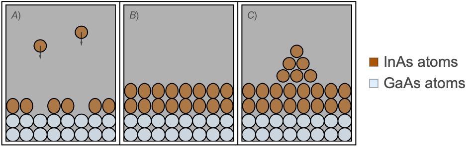
Figure 1: Depiction (not up to scale) of the SK growth methodology. Subfigure A) shows the layer-by-layer growth performed with the MBE technique. Subfigure B) shows strain building up in the first few layers by the slightly deformed ![]() . Subfigure C) shows the spontaneous formation of islands due to strain relaxation of the material.
. Subfigure C) shows the spontaneous formation of islands due to strain relaxation of the material.
After that, they can be subsequently capped by another semiconductor material that usually is the same as the substrate, obtaining the desired SQDs. Particularly, SQDs grown in the SK scheme are coupled to a thin layer, usually referred as a "wetting layer", made up mostly of the same material as the SQD. Regardless of this, and given the small relative size of the wetting layer, many theoretical studies ignore the effects of the wetting layer on the energy spectrum of the particles confined in the SQDs. Nevertheless, the suitability of not considering the wetting layer's effect on the confined eigenstates is a question worth considering.
Furthermore, the particular morphology of the grown SQD depends highly on experimental conditions in the fabrication process, such as temperature or material deposition rates [Granados, 2003]. For instance, some SQDs can have a shape that closely resembles a cone; this is the reason why in the literature such a quantum dot has been referred to as a conical quantum dot (CQD). For instance, examine Figure 2, where the region in orange represents the CQD and wetting layer coupling, composed of ![]() , and the remaining portion of the domain is composed of
, and the remaining portion of the domain is composed of ![]() .
.
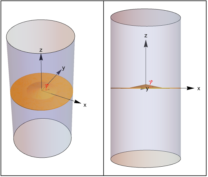
Figure 2: Depictions of a CQD, the wetting layer, and the surrounding semiconductor material from two different viewpoints. Here the ![]() vector represents the position of the electron in the Schrödinger equation.
vector represents the position of the electron in the Schrödinger equation.
As mentioned earlier, the calculations in this present document are based on the work by Melnik et al. [Melnik, 2004], which studied single electron states confined in a CQD/wetting layer structure made of the junction of ![]() and
and ![]() . In particular, this will demonstrate how to solve the time-independent Schrödinger equation and the correspondent eigenvalue problem. Consequently, this approach allows for studying the effect of the wetting layer's size on single electron states confined in this characteristic geometry. This will show some advantages of using the finite element method as implemented in the Wolfram Language.
. In particular, this will demonstrate how to solve the time-independent Schrödinger equation and the correspondent eigenvalue problem. Consequently, this approach allows for studying the effect of the wetting layer's size on single electron states confined in this characteristic geometry. This will show some advantages of using the finite element method as implemented in the Wolfram Language.
Theory
Considering the effective mass and the envelope function approximations, explained in more detail here, the time-independent Schrödinger equation for the electron's wavefunction can be written as in equation 1.
Here, ![]() is the confinement potential, which takes the value of
is the confinement potential, which takes the value of ![]() inside the CQD and wetting layer regions, and a finite constant value otherwise. Furthermore, the effective mass function,
inside the CQD and wetting layer regions, and a finite constant value otherwise. Furthermore, the effective mass function, ![]() , is a piecewise function that gives the distinct effective masses associated with each material.
, is a piecewise function that gives the distinct effective masses associated with each material.
Take note of the way the kinetic term, i.e. the diffusion term, in equation 2 is written. This way of writing the Hamiltonian is usually referred to as a BenDaniel–Duke Hamiltonian. This provides a more accurate model for the mismatch between the effective masses in each region [BenDaniel-Duke, 1966].
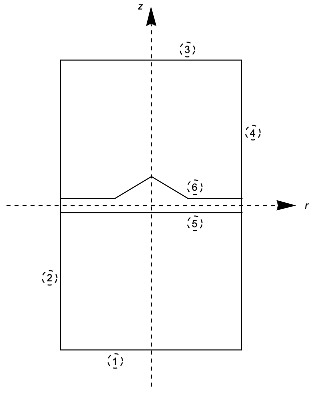
Figure 3: Cross-sectional depiction of the regions of the CQD inspired from Melnik's work [Melnik, 2004]. Numbers 1 through 6 represent each boundary surface.
In Figure 3, the entire domain for the problem is depicted through a cross-sectional view in the ![]() plane, where the numbers
plane, where the numbers ![]() through
through ![]() represent the different boundary surfaces. The volume enclosed by surfaces
represent the different boundary surfaces. The volume enclosed by surfaces ![]() and
and ![]() corresponds to the coupling between the CQD and the wetting layer, composed of
corresponds to the coupling between the CQD and the wetting layer, composed of ![]() . The rest of the domain consists of
. The rest of the domain consists of ![]() .
.
Particularly, the focus is only on bound states, i.e. states that will decay at a far enough distance from the CQD and wetting layer structure. For that reason, a Dirichlet boundary condition will be used, which ensures that ![]() on surfaces
on surfaces ![]() and
and ![]() . In contrast, as some states may disperse throughout the wetting layer, extending beyond the confinement of the CQD, Dirichlet boundary conditions are not used for surfaces
. In contrast, as some states may disperse throughout the wetting layer, extending beyond the confinement of the CQD, Dirichlet boundary conditions are not used for surfaces ![]() and
and ![]() . Instead, Neumann flux
. Instead, Neumann flux ![]() boundary conditions, where
boundary conditions, where ![]() , will be used. This will allow the wavefunction to have a nonzero value at these outer boundaries. On top of that, the BenDaniel–Duke boundary conditions need to be enforced at boundaries
, will be used. This will allow the wavefunction to have a nonzero value at these outer boundaries. On top of that, the BenDaniel–Duke boundary conditions need to be enforced at boundaries ![]() and
and ![]() , which means that this relation,
, which means that this relation, ![]() , must hold true at these internal boundaries [BenDaniel-Duke, 1966].
, must hold true at these internal boundaries [BenDaniel-Duke, 1966].
On the other hand, taking advantage of the cylindrical symmetry of the geometry, and assuming that both the confinement potential and the effective mass functions are independent of the azimuthal coordinate ![]() , the dimensionality of the problem can be reduced from 3D to 2D.
, the dimensionality of the problem can be reduced from 3D to 2D.
Start from the 3D Schrödinger equation in cylindrical coordinates:
On the assumption that the ![]() function does not depend on
function does not depend on ![]() , applying the definition of the differential operators in cylindrical coordinates leads to the following:
, applying the definition of the differential operators in cylindrical coordinates leads to the following:
Then, given the cylindrical symmetry about the ![]() axis of the CQD, the ansatz
axis of the CQD, the ansatz ![]() is proposed. This leads to:
is proposed. This leads to:
Now, by dividing the whole equation by ![]() , it is possible to separate the problem into two equations. After some rearranging and simplification, this results in:
, it is possible to separate the problem into two equations. After some rearranging and simplification, this results in:
This way, a particular solution for equation for equation 3 is:
where ![]() , the azimuthal or angular momentum quantum number, is an integer due to the periodicity
, the azimuthal or angular momentum quantum number, is an integer due to the periodicity ![]() .
.
This approach allows for solving equation 4 in a 2D geometry shown in Figure 4, obtaining the energy eigenvalues, ![]() and the 2D wavefunctions
and the 2D wavefunctions ![]() . Then, the total wavefunctions are obtained by equation 5.
. Then, the total wavefunctions are obtained by equation 5.
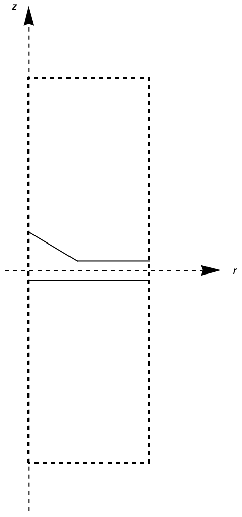
Figure 4: Working domain to solve equation 6.
Geometry
The first step to model this system is to define some parameters. All the lengths are going to be taken as nanometers.
WLWidth = 2;
dotRadius  = 12;
dotHeight = 2.6;
domainRadius = 25;
domainHeight = 100;
Here, WLWidth is the wetting layer's thickness. dotRadius and dotHeight are the base radius and height of the CQD, respectively. And domainHeight and domainRadius, are the height and width of the whole 2D region in which equation 7 will be solved, respectively.
Next, the domains are defined. Particularly, a distinction between the region for the CQD and wetting layer coupling from the rest of the region is desirable. So separate regions are defined.
QDWL = RegionUnion[Triangle[{{0, dotHeight + (WLWidth/2)}, {0, (WLWidth/2)}, {dotRadius, (WLWidth/2)}}], Rectangle[{0, -(WLWidth/2)}, {domainRadius, (WLWidth/2)}]];
RegionPlot[QDWL, ...]
For the region corresponding to the CQD, the Triangle function is used, and the Rectangle function is used for the wetting layer region. Then RegionUnion is used to create a single CQD/wetting layer region. Also, observe that the value at ![]() aligns with the midpoint of the wetting layer's width.
aligns with the midpoint of the wetting layer's width.
region = Rectangle[{0, -(domainHeight/2)}, {domainRadius, (domainHeight/2)}];
RegionPlot[region, ...]
To have more control over the quality of the solution, the mesh used for the finite element method will be generated first. This way it is possible to visualize the mesh more easily and refine it if necessary.
Is necessary to import the FEM package.
Needs["NDSolve`FEM`"]The RegionBoundary function is used to extract the boundaries of the CQD/wetting layer region and the whole domain region. Then they are combined into a boundary mesh.
bmesh = ToBoundaryMesh[RegionUnion[RegionBoundary[QDWL], RegionBoundary[region]]];
bmesh["Wireframe"]
As the focus is on obtaining the bound states, is convenient to refine the mesh where the wavefunction is more likely to take higher values, in this case, inside the CQD/wetting layer region. For that reason, the "RegionMarker" option is used in the ToElementMesh function. This way, a refinement parameter for the region with element marker ![]() is defined.
is defined.
mesh = ToElementMesh[bmesh, "RegionMarker" -> {{{(dotRadius/4), (dotHeight/2) + (WLWidth/2)}, 1, 0.25}, {{2dotRadius, 3 WLWidth}, 2}, {{2dotRadius, -3 WLWidth}, 3}}];
mesh["Wireframe"["MeshElementStyle" -> {FaceForm[Orange], FaceForm[White], FaceForm[White]}]]
Note that the mesh is more refined in the CQD/wetting layer region.
Hamiltonian
In this next step, it is necessary to generate the PDE operator. For that purpose, the potential and effective mass functions are defined.
The confinement potential is produced by the difference between the energy gaps of each material. For the junction of ![]() and
and ![]() , the potential barrier can be approximated by the value of V0=
, the potential barrier can be approximated by the value of V0=![]() [Melnik, 2004].
[Melnik, 2004].
Taking advantage of the element markers used in the mesh definition earlier, they are used to define the confinement potential.
V0 = 697;
V = Quantity[ Piecewise[{{V0, ElementMarker != 1}}], "Millielectronvolts"]
The effective masses are ![]() and
and ![]() for
for ![]() and
and ![]() , respectively [Yu, 2010], where
, respectively [Yu, 2010], where ![]() is the conventional electron mass.
is the conventional electron mass.
m0 = QuantityMagnitude[Entity["Particle", "Electron"][EntityProperty["Particle", "Mass"]], "Kilograms"];mass = Quantity[m0 Piecewise[{{0.023, ElementMarker == 1}}, 0.067], "Kilograms"];The goal is to solve equation 8. Then, to generate the correspondent PDE operator, the SchrodingerPDEComponent function is used.
pars = <|"Mass" -> mass, "SchrodingerPotential" -> V, "ScaleUnits" -> {"Meters" -> "Nanometers"}, "RegionSymmetry" -> "Axisymmetric", "AzimuthalQuantumNumber" -> l|>ℋ = SchrodingerPDEComponent[{ψ[r, z], {r, z}}, pars]It is worth mentioning the use of the parameters "RegionSymmetry" -> "Axisymmetric" and "AzimuthalQuantumNumber" -> l. With these two parameters, the SchrodingerPDEComponent yields the correspondent expressions for the terms ![]() and
and ![]() in equation 9. Also, since all geometric parameters are defined in nanometers, the parameter "ScaleUnits"{"Meters""Nanometers"} is used. This implies that the model parameters have been converted, resulting in the transformation of length units from "Meters" to "Nanometers". This ensures that the PDE operator is correctly generated by the SchrodingerPDEComponent function.
in equation 9. Also, since all geometric parameters are defined in nanometers, the parameter "ScaleUnits"{"Meters""Nanometers"} is used. This implies that the model parameters have been converted, resulting in the transformation of length units from "Meters" to "Nanometers". This ensures that the PDE operator is correctly generated by the SchrodingerPDEComponent function.
Boundary Conditions and Eigenvalue Problem Solution
As discussed earlier, a Dirichlet condition is set such that only bound states in the CQD/wetting layer region are found.
bc = DirichletCondition[ψ[r, z] == 0, z == (domainHeight/2) || z == -(domainHeight/2)];Also, as mentioned before, a Neumann flux ![]() boundary condition must be applied to boundary
boundary condition must be applied to boundary ![]() in Figure 2. In this case, there is no need to define explicitly this boundary condition, since its applied by default; see NeumannValue for details. Also, the quantity
in Figure 2. In this case, there is no need to define explicitly this boundary condition, since its applied by default; see NeumannValue for details. Also, the quantity ![]() is continuous by default between internal boundaries, which means that the BenDaniel–Duke boundary condition is correctly applied as well.
is continuous by default between internal boundaries, which means that the BenDaniel–Duke boundary condition is correctly applied as well.
At this point, NDEigensystem is used to solve the eigenvalue problem. Start by exploring the first 5 low-lying eigenstates for ![]() .
.
{en, funs} = NDEigensystem[{ℋ /. {l -> 0}, bc}, ψ[r, z], {r, z}∈mesh, 5]First of all, it is necessary to transform the energies into the correct energy units. Given that the model's parameter length units are ![]() , the energy units are the "SIBase" units for energy, but with the exception of changing
, the energy units are the "SIBase" units for energy, but with the exception of changing ![]() to
to ![]() .
.
en = UnitConvert[UnitConvert[en Quantity[1, "Joules"], "SIBase"] /. "Meters" -> "Nanometers", "Millielectronvolts"]Then, visualize the probability densities associated with the wavefunctions ![]() from equations 10 and 11, corresponding to the variable funs[[i]].
from equations 10 and 11, corresponding to the variable funs[[i]].
Table[Show[DensityPlot[funs[[i]]^2, {r, z}∈region, ...], bmesh["Wireframe"["MeshElementStyle" -> Directive[White]]], Rule[...]], {i, Length[en]}]Table[SliceDensityPlot3D[funs[[i]]^2 /. {r -> Sqrt[x^2 + y^2]}, "CenterPlanes", {x, -25, 25}, {y, -25, 25}, {z, -12, 12}, ...], {i, Length[en]}]A few comments can be made about the plots. First of all, the ground state is confined mainly in the center of the CQD, as expected. And on the other hand, for the rest of the states, the probability densities are much more spread on the wetting layer than the ground state.
The Effect of the Azimuthal Quantum Number
To explore the effect of introducing the azimuthal quantum number, the value of ![]() is set to 1 and the eigenvalue problem is solved in a similar fashion as before. The choice of that specific value for
is set to 1 and the eigenvalue problem is solved in a similar fashion as before. The choice of that specific value for ![]() will become clear later.
will become clear later.
{en, funs} = NDEigensystem[{ℋ /. {l -> 1}, bc}, ψ[r, z], {r, z}∈mesh, 5]en = UnitConvert[UnitConvert[en Quantity[1, "Joules"], "SIBase"] /. "Meters" -> "Nanometers", "Millielectronvolts"]In the case with ![]() , the last eigenvalue is larger than the potential barrier, which is V0=
, the last eigenvalue is larger than the potential barrier, which is V0=![]() , and therefore is an unbounded state. This can be verified by plotting the probability densities.
, and therefore is an unbounded state. This can be verified by plotting the probability densities.
One thing to be aware of is that by setting ![]() to a nonzero value, the wavefunction is
to a nonzero value, the wavefunction is ![]() instead of just
instead of just ![]() , which means that the i th state will be represented by the expression funs[[i]]Exp[lϕ]; therefore, the wavefunction is now complex valued. Regardless of that, the probability density still is
, which means that the i th state will be represented by the expression funs[[i]]Exp[lϕ]; therefore, the wavefunction is now complex valued. Regardless of that, the probability density still is ![]() , and therefore, the i th probability density is represented by funs[[i]]2.
, and therefore, the i th probability density is represented by funs[[i]]2.
Table[Show[DensityPlot[funs[[i]]^2, {r, z}∈region, ...], bmesh["Wireframe"["MeshElementStyle" -> Directive[White]]], Rule[...]], {i, Length[en]}]Here lies an interesting aspect of introducing the azimuthal quantum number. First of all, the fifth eigenstate is unbounded, as anticipated. Furthermore, the probability density is ![]() at
at ![]() for all the eigenstates. Particularly, the term
for all the eigenstates. Particularly, the term ![]() in equation 12 explains this behavior, as this is a repulsion term. As
in equation 12 explains this behavior, as this is a repulsion term. As ![]() tends to
tends to ![]() , this term approaches infinity, which forces the wavefunction, and therefore the probability density, to decay to
, this term approaches infinity, which forces the wavefunction, and therefore the probability density, to decay to ![]() at
at ![]() . Also, notice that this effect is absent for l=0, as seen in the respective probability densities. This behavior will be noticed for any nonzero value of
. Also, notice that this effect is absent for l=0, as seen in the respective probability densities. This behavior will be noticed for any nonzero value of ![]() , and for that reason, any value for which
, and for that reason, any value for which ![]() could have been chosen.
could have been chosen.
Plot[(1/r^2), {r, 0, 25}, ...]On the other hand, it is also possible to visualize the complete wavefunction with DensityPlot3D. To do that, it is necessary to take into account that introducing a nonzero value for ![]() makes the wavefunction complex valued. Therefore, it is necessary to plot the imaginary and real parts separately.
makes the wavefunction complex valued. Therefore, it is necessary to plot the imaginary and real parts separately.
Table[Row[DensityPlot3D[# /. {r -> Sqrt[x^2 + y^2], ϕ -> ArcTan[x, y], l -> 1}, {x, -25, 25}, {y, -25, 25}, {z, -30, 30}, RegionFunction -> (!(#1 > 0 && #2 < 0)&), ...]& /@ {Re[Exp[I l ϕ]funs[[i]]], Im[Exp[I l ϕ]funs[[i]]]}], {i, Length[en]}]On the other hand, the effect of changing ![]() on the energy eigenvalues can be explored. To do that, a helper function is defined to solve the eigenvalue problem for each value of
on the energy eigenvalues can be explored. To do that, a helper function is defined to solve the eigenvalue problem for each value of ![]() .
.
AzimuthalQuantumNumberEigenvalues[AzimuthalQuantumNumber_Integer] := Module[{en, l0 = AzimuthalQuantumNumber},
	en = NDEigenvalues[{ℋ /. {l -> l0}, bc}, ψ[r, z], {r, z}∈mesh, 5];
	en = UnitConvert[UnitConvert[en Quantity[1, "Joules"], "SIBase"] /. "Meters" -> "Nanometers", "Millielectronvolts"]
]AzimuthalQuantumNumberEnergies = Table[{l, #}& /@ AzimuthalQuantumNumberEigenvalues[l], {l, -5, 5, 1}];ListPlot[AzimuthalQuantumNumberEnergies, ...]In the plot of the energy eigenvalues for different values of ![]() raging from
raging from ![]() to
to ![]() , it is possible to see that the larger the absolute value of
, it is possible to see that the larger the absolute value of ![]() , the larger the energy eigenvalues. This can be explained by thinking about
, the larger the energy eigenvalues. This can be explained by thinking about ![]() as the angular momentum quantum number. The quantum mechanical operator associated with the angular momentum around the
as the angular momentum quantum number. The quantum mechanical operator associated with the angular momentum around the ![]() axis, which is the axis of symmetry for the CQD/wetting layer structure, is written in equation 13.
axis, which is the axis of symmetry for the CQD/wetting layer structure, is written in equation 13.
It can be easily checked that the wavefunction from equation 14, ![]() , is an eigenfunction of the operator
, is an eigenfunction of the operator ![]() in equation 15. Therefore, according to quantum theory, the correspondent eigenvalues
in equation 15. Therefore, according to quantum theory, the correspondent eigenvalues ![]() represent the possible values for the angular momentum with respect to the
represent the possible values for the angular momentum with respect to the ![]() axis. Consequently, higher values of
axis. Consequently, higher values of ![]() directly correspond to states possessing greater angular momentum relative to the
directly correspond to states possessing greater angular momentum relative to the ![]() axis. This in turn gives a physical explanation for the higher energy eigenvalues observed with increasing
axis. This in turn gives a physical explanation for the higher energy eigenvalues observed with increasing ![]() values.
values.
On the other hand, as can be seen in the plot above, where the horizontal red line represents the barrier height V0=![]() , for larger values of
, for larger values of ![]() , fewer states are bounded in the CQD/wetting layer region. Since these are more energetic states, more unbounded states are expected.
, fewer states are bounded in the CQD/wetting layer region. Since these are more energetic states, more unbounded states are expected.
The Effect of the Wetting Layer's Size
To study the effect of changing the wetting layer's size, the geometrical parameters will be fixed except the wetting layer's width.
{WLWidth, dotRadius, dotHeight, domainRadius, domainHeight}Next, the eigenvalues will be calculated as a function of the wetting layer's width for an axisymmetric quantum number of ![]() for simplicity, since the effect of changing
for simplicity, since the effect of changing ![]() has already been explored above. If readers are interested in observing the effect of changing both
has already been explored above. If readers are interested in observing the effect of changing both ![]() and the wetting layer's width, they can modify the following helper function defined to calculate the eigenvalues as a function of the WLWidth parameter.
and the wetting layer's width, they can modify the following helper function defined to calculate the eigenvalues as a function of the WLWidth parameter.
WLWidthEigenstates[WLWidth_] := Module[{en, funs, QDWL, bmesh, mesh, V, mass, ℋ},
	QDWL = RegionUnion[Triangle[{{0, dotHeight + (WLWidth/2)}, {0, (WLWidth/2)}, {dotRadius, (WLWidth/2)}}], Rectangle[{0, -(WLWidth/2)}, {domainRadius, (WLWidth/2)}]];

	bmesh = ToBoundaryMesh[RegionUnion[RegionBoundary[QDWL], RegionBoundary[region]]];
	mesh = ToElementMesh[bmesh, "RegionMarker" -> {{{(dotRadius/4), (dotHeight/2) + (WLWidth/2)}, 1, 0.25}, {{2dotRadius, 3 WLWidth}, 2}, {{2dotRadius, -3 WLWidth}, 3}}];

	V = Quantity[ Piecewise[{{V0, ElementMarker != 1}}], "Millielectronvolts"];mass = Quantity[m0 Piecewise[{{0.023, ElementMarker == 1}}, 0.067], "Kilograms"];

	ℋ = SchrodingerPDEComponent[{ψ[r, z], {r, z}}, <|"Mass" -> mass, "SchrodingerPotential" -> V, "ScaleUnits" -> {"Meters" -> "Nanometers"}, "RegionSymmetry" -> "Axisymmetric", "AzimuthalQuantumNumber" -> l|>];

	{en, funs} = NDEigensystem[{ℋ /. {l -> 0}, bc}, ψ[r, z], {r, z}∈mesh, 5];
	en = UnitConvert[UnitConvert[en Quantity[1, "Joules"], "SIBase"] /. "Meters" -> "Nanometers", "Millielectronvolts"];
	{en, funs}
	]
Note that to calculate the energy eigenvalues for different geometrical configurations, one must generate a new mesh and redefine the confinement potential and effective mass functions.
WLWidthStates = Table[{Map[ Function[En, {WL, En}], #[[1]]], {WL, #[[2]]}}&[WLWidthEigenstates[WL]] , {WL, 0, 2.5, 0.25}];ListPlot[WLWidthStates[[All, 1]], ...]In the later plot, some degeneracies in the energy eigenvalues can be observed for lower values of the wetting layer's width, such as states ![]() and
and ![]() being degenerate for values of the parameter WLWidth from
being degenerate for values of the parameter WLWidth from ![]() up to
up to ![]() . Then, these degeneracies are gone for subsequent higher values of the wetting layer's width. Moreover, for values of the wetting layer's width of
. Then, these degeneracies are gone for subsequent higher values of the wetting layer's width. Moreover, for values of the wetting layer's width of ![]() and
and ![]() the fifth state is a bound state, unlike with lower values of WLWidth.
the fifth state is a bound state, unlike with lower values of WLWidth.
Overall, the eigenvalues decrease monotonically as the wetting layer's width increases. This is expected, since the total volume where the electron is being confined is growing. In light of Heisenberg's uncertainty principle, when the wetting layer's width value is small, the wavefunction is more packed, and therefore the uncertainty in the position is lowest, which implies that the uncertainty in the momentum is highest. In other words, as the particle is more confined, its mean square momentum is larger and then its kinetic energy will be larger as well. This explains why the energy eigenvalues are higher for lower values of the wetting layer's width. On the other hand, the opposite effect also occurs, as the wetting layer grows, the wavefunction becomes more spread out and the uncertainty in the position increases, causing the uncertainty in the momentum to decrease. Then, the mean square momentum is lower, which implies a lower kinetic energy for the particle for higher values of the wetting layer's width.
To verify this reasoning, the probability densities are compared. For the bound states, between the results for a wetting layer width of ![]() and those with a wetting layer width of
and those with a wetting layer width of ![]() . Only the first three states are chosen because they are the only bound states for a wetting layer width of
. Only the first three states are chosen because they are the only bound states for a wetting layer width of ![]() .
.
funsSmallerWL = Cases[WLWidthStates[[All, 2]], {0.25, ___}][[1, 2]]funsLargerWL = Cases[WLWidthStates[[All, 2]], {2.5, ___}][[1, 2]]Note that to plot the wavefunction corresponding to different geometrical parameters, the mesh is extracted from each solution.
Table[Show[DensityPlot[Abs[#[[i]]], {r, z}∈Head[#[[i]]]["ElementMesh"], ...], Head[#[[i]]]["ElementMesh"]["Wireframe"["MeshElement" -> "BoundaryElements", "MeshElementStyle" -> Directive[White]]], Rule[...]]& /@ {funsSmallerWL, funsLargerWL}, {i, 3}];
Column[Row /@ %]
In the plot above, the probability density for the first three bound states is plotted. The left and right columns correspond to values of the WLWidth parameter of ![]() and
and ![]() , respectively. It is noticeable that for the smaller wetting layer width value, the probability density is compressed and exhibits greater localization, specially for the low-lying states, compared to the wavefunctions for a larger wetting layer, as expected.
, respectively. It is noticeable that for the smaller wetting layer width value, the probability density is compressed and exhibits greater localization, specially for the low-lying states, compared to the wavefunctions for a larger wetting layer, as expected.
Conclusion
The impact of the azimuthal quantum number and the thickness of the wetting layer has been investigated on the eigenstates of a mono-electronic system confined within a CQD coupled to a wetting layer. It was observed that the introduction of the azimuthal quantum number leads to the wavefunction vanishing at the axis of symmetry. Moreover, as the value of the azimuthal quantum number increases, so do the energy eigenvalues.
On the other hand, a decrease in the energy eigenvalues was noted with an increase in the width of the wetting layer, consistent with the anticipated behavior, as discussed earlier. This emphasizes the significant influence of the wetting layer's size on the energy eigenvalues and highlights the importance of incorporating it into the model.
In this overview, the essential methodology has been explained for those interested in solving similar problems using the Wolfram Language.
References
1. Seravalli, L. (2023). "Metamorphic InAs/InGaAs Quantum Dots for Optoelectronic Devices: A Review." Microelectronic Engineering, 276, 111996. https://doi.org/10.1016/j.mee.2023.111996.
2. Sogabe, T., Shoji, Y., Miyashita, N., Farrell, D. J., Shiba, K., Hong, H.-F. & Okada, Y. (2023). "High-Efficiency InAs/GaAs Quantum Dot Intermediate Band Solar Cell Achieved through Current Constraint Engineering." Next Materials, 1(2), 100013. https://doi.org/10.1016/j.nxmate.2023.100013.
3. Yu, P. Y. & Cardona, M. (2010). Fundamentals of Semiconductors (pp. 8–13). https://doi.org/10.1007/978-3-642-00710-1.
4. Granados, D. and Garcia, J. M. (2003). "Customized Nanostructures MBE Growth: From Quantum Dots to Quantum Rings." Journal of Crystal Growth, 251(1–4), pp. 213–217. https://doi.org/10.1016/S0022-0248(02)02512-5.
5. Melnik, R. V. N. and Willatzen, M. (2004). Bandstructures of Conical Quantum Dots with Wetting Layers." Nanotechnology, 15(1), pp. 1–8. https://doi.org/10.1088/0957-4484/15/1/001.
6. BenDaniel, D. J. and Duke, C. B. (1966). "Space-Charge Effects on Electron Tunneling." Physical Review, 152(2), pp. 683–692. https://doi.org/10.1103/PhysRev.152.683.