


DensityPlot3D
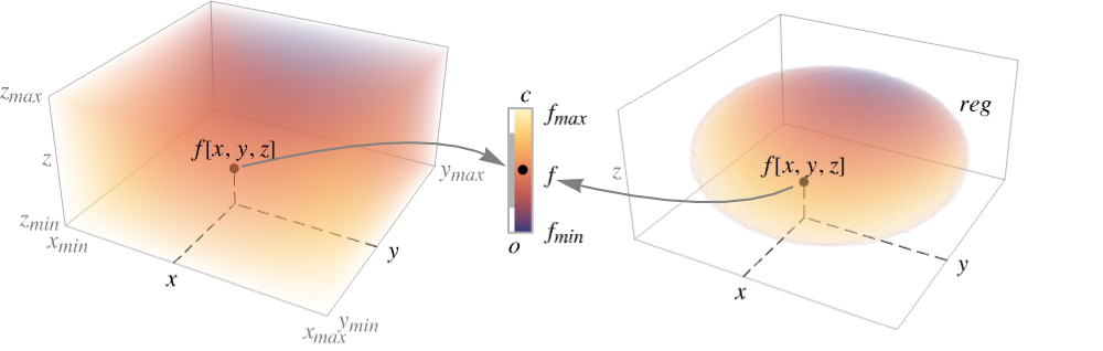
DensityPlot3D[f,{x,xmin,xmax},{y,ymin,ymax},{z,zmin,zmax}]
makes a density plot of f as a function of x, y, and z.
DensityPlot3D[f,{x,y,z}∈reg]
takes the variables to be in the geometric region reg.
Details and Options
- DensityPlot3D is also known as volume map.
- DensityPlot3D evaluates the function
 over its domain and maps the value to a color and opacity independently.
 - The opacity function
 is typically used to make some range of values visible, while making some others invisible.
 - The plot visualizes the set
 , where
  is a color function and
  is an opacity function.
 - At positions where f does not evaluate to a real number, data is taken to be missing and is rendered transparently.
- DensityPlot3D treats the variables x, y, and z as local, effectively using Block.
- DensityPlot3D has attribute HoldAll, and evaluates f only after assigning specific numerical values to x, y, and z.
- In some cases it may be more efficient to use Evaluate to evaluate f symbolically before specific numerical values are assigned to x, y, and z.
- DensityPlot3D has the same options as Graphics3D, with the following additions and changes: [List of all options]
-
Axes True whether to draw axes BoxRatios {1,1,1} bounding 3D box ratios ColorFunction Automatic how to color the plot ColorFunctionScaling True whether to scale the arguments to ColorFunction OpacityFunction Automatic how to compute the opacity at each point OpacityFunctionScaling True whether to scale the arguments to OpacityFunction PerformanceGoal $PerformanceGoal aspects of performance to optimize PlotLegends None legends for color gradients PlotPoints Automatic initial number of samples for the function in each direction PlotRange {Full,Full,Full,Automatic} range of f or other values to include PlotTheme $PlotTheme overall theme for the plot RegionFunction (True&) how to determine whether a point should be included ScalingFunctions None how to scale individual coordinates TargetUnits Automatic desired units to use WorkingPrecision MachinePrecision the precision used in internal computations - ColorFunction and OpacityFunction are supplied with a single argument, given by default by the scaled value of f.
- Typical settings for OpacityFunction include:
-
Automatic automatically determined None no opacity function, fully opaque α constant opacity Opacity[α] Interval[…] make values in the interval more opaque "Image3D" default opacity function used in Image3D func general opacity function - The arguments supplied to RegionFunction are x, y, z, and f.
- Possible settings for ScalingFunctions include:
-
sf scale the fcontour values {sx,sy,sz} scale x, y and z axes {sx,sy,sz,sf} scale x, y and z axes and fcontour values - Common built-in scaling functions s include:
-
"Log" 
log scale with automatic tick labeling "Log10" 
base-10 log scale with powers of 10 for ticks "SignedLog" 
log-like scale that includes 0 and negative numbers "Reverse" 
reverse the coordinate direction "Infinite" 
infinite scale
List of all options
Examples
open all close allBasic Examples (3)
DensityPlot3D[x y z, {x, -1, 1}, {y, -1, 1}, {z, -1, 1}]DensityPlot3D[Sin[x]Cos[y]Sin[z], {x, y, z}∈Ball[{0, 0, 0}, 5], PlotTheme -> "Marketing"]Use a different color scheme and legend:
f = PDF[DirichletDistribution[{1, 2, 3, 4}], {x, y, z}]DensityPlot3D[f, {x, 0, 0.5}, {y, 0, 1}, {z, 0, 1}, ColorFunction -> "SunsetColors", PlotLegends -> Automatic]Scope (13)
Sampling (6)
Areas where the function becomes nonreal are excluded:
DensityPlot3D[Sqrt[x y z], {x, y, z}∈Ball[], OpacityFunction -> None]Use PlotPoints to control sampling:
Table[DensityPlot3D[x y z, {x, -1, 1}, {y, -1, 1}, {z, -1, 1}, PlotPoints -> pp], {pp, {5, 20, 50}}]The domain may be specified by a region including Cone:
DensityPlot3D[x y z, {x, y, z}∈Cone[]]A formula region including ImplicitRegion:
ℛ = ImplicitRegion[(x ^ 2 + (9 / 4)y ^ 2 + z ^ 2 - 1) ^ 3 - x ^ 2z ^ 3 - (9 / 80)y ^ 2z ^ 3 <= 0, {{x, -1.2, 1.2}, {y, -0.7, 0.7}, {z, -1, 1.3}}];DensityPlot3D[x y z, {x, y, z}∈ℛ]A mesh-based region including BoundaryMeshRegion:
ℛ = ConvexHullMesh[RandomReal[1, {25, 3}]]DensityPlot3D[x y z, {x, y, z}∈ℛ]Use PlotRange to limit ranges to expose more detail:
DensityPlot3D[Exp[-(x ^ 2 + y ^ 2 + z ^ 2)], {x, -1, 1}, {y, -1, 1}, {z, -1, 1}, PlotRange -> {{-1, 0}, All, All}, BoxRatios -> Automatic]Use ClipPlanes to specify one or several clipping planes. In this case, clip ![]() :
:
DensityPlot3D[Sin[x + y + z] / 10, {x, 0, 10}, {y, 0, 10}, {z, 0, 10}, OpacityFunction -> None, ClipPlanes -> {1, 1, -1, 0}]Use RegionFunction to constrain point inclusion more generally:
DensityPlot3D[x ^ 2 + y ^ 2 - z ^ 2, {x, -2, 2}, {y, -2, 2}, {z, -2, 2}, RegionFunction -> Function[{x, y, z, f}, x < y ^ 3]]Presentation (7)
Use PlotTheme to immediately get overall styling:
Table[DensityPlot3D[x y z, {x, -1, 1}, {y, -1, 1}, {z, -1, 1}, PlotLabel -> t, PlotTheme -> t], {t, {"Minimal", "Scientific", "Marketing"}}]Use PlotLegends to get a color bar for the different values:
DensityPlot3D[x y z, {x, -1, 1}, {y, -1, 1}, {z, -1, 1}, PlotLegends -> Automatic]Control the display of axes with Axes:
Table[DensityPlot3D[x y z, {x, -1, 1}, {y, -1, 1}, {z, -1, 1}, PlotLabel -> a, Axes -> a], {a, {True, False, {True, False, True}}}]Label axes using AxesLabel and the whole plot using PlotLabel:
DensityPlot3D[x y z, {x, -1, 1}, {y, -1, 1}, {z, -1, 1}, Ticks -> None, AxesLabel -> {x, y, z}, PlotLabel -> x y z]Color the plot by the function values with ColorFunction:
Table[DensityPlot3D[x y z, {x, -1, 1}, {y, -1, 1}, {z, -1, 1}, PlotLabel -> c, ColorFunction -> c], {c, {Hue, "BlueGreenYellow"}}]TargetUnits specifies which units to use in the visualization:
DensityPlot3D[Quantity[x y z, "kg/m^3"], {x, -1, 1}, {y, -1, 1}, {z, -1, 1}, AxesLabel -> Automatic, PlotLegends -> Automatic, TargetUnits -> {"Feet", "Feet", "Feet", "g/ft^3"}]DensityPlot3D[Sin[2π x]Sin[2π y] + z, {x, 0, 1}, {y, 0, 1}, {z, 0, 1}, ScalingFunctions -> {"Log", None, None}]Reverse the ![]() axis so that values increase as they go down:
axis so that values increase as they go down:
DensityPlot3D[Sin[2π x]Sin[2π y] + z, {x, 0, 1}, {y, 0, 1}, {z, 0, 1}, ScalingFunctions -> {None, None, "Reverse"}]Options (69)
Axes (4)
By default, axes are drawn for DensityPlot3D:
DensityPlot3D[Sin[2π x]Sin[2π y]Sin[2π z], {x, -1, 1}, {y, -1, 1}, {z, -1, 1}]Use AxesFalse to turn off axes:
DensityPlot3D[Sin[2π x]Sin[2π y]Sin[2π z], {x, -1, 1}, {y, -1, 1}, {z, -1, 1}, Axes -> False]Use AxesOrigin to specify where the axes intersect:
DensityPlot3D[Sin[2π x]Sin[2π y]Sin[2π z], {x, -1, 1}, {y, -1, 1}, {z, -1, 1}, AxesOrigin -> {0, 0, 0}]Turn each axis on individually:
{DensityPlot3D[Sin[2π x]Sin[2π y]Sin[2π z], {x, -1, 1}, {y, -1, 1}, {z, -1, 1}, Axes -> {False, False, True}], DensityPlot3D[Sin[2π x]Sin[2π y]Sin[2π z], {x, -1, 1}, {y, -1, 1}, {z, -1, 1}, Axes -> {True, False, False}], DensityPlot3D[Sin[2π x]Sin[2π y]Sin[2π z], {x, -1, 1}, {y, -1, 1}, {z, -1, 1}, Axes -> {False, True, False}]}AxesLabel (4)
No axes labels are drawn by default:
DensityPlot3D[Sin[2π x]Sin[2π y]Sin[2π z], {x, -1, 1}, {y, -1, 1}, {z, -1, 1}]DensityPlot3D[Sin[2π x]Sin[2π y]Sin[2π z], {x, -1, 1}, {y, -1, 1}, {z, -1, 1}, AxesLabel -> z]DensityPlot3D[Sin[2π x]Sin[2π y]Sin[2π z], {x, -1, 1}, {y, -1, 1}, {z, -1, 1}, AxesLabel -> {"X", "Y", "Z"}]Use labels based on variables specified in DensityPlot3D:
DensityPlot3D[Sin[2π x]Sin[2π y]Sin[2π z], {x, -1, 1}, {y, -1, 1}, {z, -1, 1}, AxesLabel -> Automatic]AxesOrigin (2)
The position of the axes is determined automatically:
DensityPlot3D[Sin[2π x]Sin[2π y]Sin[2π z], {x, -1, 1}, {y, -1, 1}, {z, -1, 1}]Specify an explicit origin for the axes:
DensityPlot3D[Sin[2π x]Sin[2π y]Sin[2π z], {x, -1, 1}, {y, -1, 1}, {z, -1, 1}, AxesOrigin -> {0, 0, 0}]AxesStyle (4)
Change the style for the axes:
DensityPlot3D[Sin[2π x]Sin[2π y]Sin[2π z], {x, -1, 1}, {y, -1, 1}, {z, -1, 1}, AxesStyle -> Red]Specify the style of each axis:
DensityPlot3D[Sin[2π x]Sin[2π y]Sin[2π z], {x, -1, 1}, {y, -1, 1}, {z, -1, 1}, AxesStyle -> {{Thick, Brown}, {Thick, Blue}, {Thick, Green}}]Use different styles for the ticks and the axes:
DensityPlot3D[Sin[2π x]Sin[2π y]Sin[2π z], {x, -1, 1}, {y, -1, 1}, {z, -1, 1}, AxesStyle -> Green, TicksStyle -> StandardBlue]Use different styles for the labels and the axes:
DensityPlot3D[Sin[2π x]Sin[2π y]Sin[2π z], {x, -1, 1}, {y, -1, 1}, {z, -1, 1}, AxesStyle -> Green, LabelStyle -> StandardBlue]BoxRatios (2)
By default, the edges of the bounding box have the same length:
DensityPlot3D[Sin[x ]Cos[y] Sin[z], {x, -Pi / 2, 3Pi / 2}, {y, -Pi / 2, 3Pi / 2}, {z, -3Pi, 3Pi}]Use BoxRatios->Automatic to show the natural scale of the 3D coordinate values:
DensityPlot3D[Sin[x ]Cos[y] Sin[z], {x, -Pi / 2, 3Pi / 2}, {y, -Pi / 2, 3Pi / 2}, {z, -3Pi, 3Pi}, BoxRatios -> Automatic]ClipPlanes (3)
Use ClipPlanes to specify one or several clipping planes. In this case, clip ![]() :
:
DensityPlot3D[Sin[x + y + z] / 10, {x, 0, 10}, {y, 0, 10}, {z, 0, 10}, OpacityFunction -> None, ClipPlanes -> {{1, 1, -1, 0}}]Specify several clip planes, in this case clipping ![]() and
and ![]() :
:
DensityPlot3D[Sin[x + y + z] / 10, {x, 0, 10}, {y, 0, 10}, {z, 0, 10}, OpacityFunction -> None, ClipPlanes -> {{1, 1, -1, 0}, {0, 1, 0, -4}}]Compare to the general RegionFunction:
DensityPlot3D[Sin[x + y + z] / 10, {x, 0, 10}, {y, 0, 10}, {z, 0, 10}, OpacityFunction -> None, RegionFunction -> Function[{x, y, z}, x + y - z ≥ 0]]ColorFunction (1)
ColorFunctionScaling (2)
Parameters to ColorFunction are normally scaled to be between 0 and 1:
DensityPlot3D[x + y + z, {x, 0, 3}, {y, 0, 3}, {z, 0, 3}, ColorFunction -> Hue]Use unscaled density values by setting ColorFunctionScaling to False:
DensityPlot3D[Sin[2x y z], {x, -2, 2}, {y, -2, 2}, {z, -2, 2}, ColorFunction -> (If[# < 0, Red, Green]&), ColorFunctionScaling -> False, PlotPoints -> 100]ImageSize (7)
Use named sizes such as Tiny, Small, Medium and Large:
{DensityPlot3D[Sin[2π x]Sin[2π y]Sin[2π z], {x, -1, 1}, {y, -1, 1}, {z, -1, 1}, ImageSize -> Tiny], DensityPlot3D[Sin[2π x]Sin[2π y]Sin[2π z], {x, -1, 1}, {y, -1, 1}, {z, -1, 1}, ImageSize -> Small]}Specify the width of the plot:
{DensityPlot3D[Sin[2π x]Sin[2π y]Sin[2π z], {x, -1, 1}, {y, -1, 1}, {z, -1, 1}, ImageSize -> 150], DensityPlot3D[Sin[2π x]Sin[2π y]Sin[2π z], {x, -1, 1}, {y, -1, 1}, {z, -1, 1}, AspectRatio -> 1.5, ImageSize -> 150]}Specify the height of the plot:
{DensityPlot3D[Sin[2π x]Sin[2π y]Sin[2π z], {x, -1, 1}, {y, -1, 1}, {z, -1, 1}, ImageSize -> {Automatic, 150}], DensityPlot3D[Sin[2π x]Sin[2π y]Sin[2π z], {x, -1, 1}, {y, -1, 1}, {z, -1, 1}, AspectRatio -> 2, ImageSize -> {Automatic, 150}]}Allow the width and height to be up to a certain size:
{DensityPlot3D[Sin[2π x]Sin[2π y]Sin[2π z], {x, -1, 1}, {y, -1, 1}, {z, -1, 1}, ImageSize -> UpTo[200]], DensityPlot3D[Sin[2π x]Sin[2π y]Sin[2π z], {x, -1, 1}, {y, -1, 1}, {z, -1, 1}, AspectRatio -> 2, ImageSize -> UpTo[200]]}Specify the width and height for a graphic, padding with space if necessary:
DensityPlot3D[Sin[2π x]Sin[2π y]Sin[2π z], {x, -1, 1}, {y, -1, 1}, {z, -1, 1}, ImageSize -> {200, 300}, Background -> StandardGray]Setting AspectRatioFull will fill the available space:
DensityPlot3D[Sin[2π x]Sin[2π y]Sin[2π z], {x, -1, 1}, {y, -1, 1}, {z, -1, 1}, AspectRatio -> Full, ImageSize -> {200, 300}, Background -> StandardGray]Use maximum sizes for the width and height:
{DensityPlot3D[Sin[2π x]Sin[2π y]Sin[2π z], {x, -1, 1}, {y, -1, 1}, {z, -1, 1}, ImageSize -> {UpTo[150], UpTo[100]}], DensityPlot3D[Sin[2π x]Sin[2π y]Sin[2π z], {x, -1, 1}, {y, -1, 1}, {z, -1, 1}, AspectRatio -> 2, ImageSize -> {UpTo[150], UpTo[100]}]}Use ImageSizeFull to fill the available space in an object:
Framed[Pane[DensityPlot3D[Sin[2π x]Sin[2π y]Sin[2π z], {x, -1, 1}, {y, -1, 1}, {z, -1, 1}, ImageSize -> Full, Background -> StandardGray], {200, 100}]]Specify the image size as a fraction of the available space:
Framed[Pane[DensityPlot3D[Sin[2π x]Sin[2π y]Sin[2π z], {x, -1, 1}, {y, -1, 1}, {z, -1, 1}, AspectRatio -> Full, ImageSize -> {Scaled[0.5], Scaled[0.5]}, Background -> StandardGray], {200, 200}]]OpacityFunction (6)
OpacityFunction is Automatic by default:
DensityPlot3D[x y z, {x, -1, 1}, {y, -1, 1}, {z, -1, 1}]Turn off transparency with OpacityFunctionNone:
DensityPlot3D[x y z, {x, -1, 1}, {y, -1, 1}, {z, -1, 1}, OpacityFunction -> None]Make values in the intervals ![]() and
and ![]() more opaque:
more opaque:
DensityPlot3D[Sin[π x]Sin[π y] Sin[π z], {x, -1, 1}, {y, -1, 1}, {z, -1, 1}, OpacityFunction -> Interval[{-1, -0.6}, {0.6, 1}], OpacityFunctionScaling -> False, PlotLegends -> Automatic]Use a constant opacity Opacity[0.05]:
DensityPlot3D[Sin[π x]Sin[π y] Sin[π z], {x, -1, 1}, {y, -1, 1}, {z, -1, 1}, OpacityFunction -> 0.05, PlotLegends -> Automatic]Use the same opacity function as the one used in Image3D:
f = PDF[DirichletDistribution[{1, 2, 3, 4}], {x, y, z}];DensityPlot3D[f, {x, 0, 1}, {y, 0, 1}, {z, 0, 1}, OpacityFunction -> "Image3D", PlotLegends -> Automatic]Use a custom opacity function to specify the opacity for each density value:
DensityPlot3D[x y z, {x, -1, 1}, {y, -1, 1}, {z, -1, 1}, OpacityFunction -> Function[f, (1 - f) ^ 2]]OpacityFunctionScaling (3)
By default, scaled values are used:
DensityPlot3D[x y z, {x, -1, 1}, {y, -1, 1}, {z, -1, 1}, OpacityFunction -> Function[f, (1 - f) ^ 2]]Use unscaled density values by setting OpacityFunctionScaling to False:
DensityPlot3D[x + y + z, {x, -1, 1}, {y, -1, 1}, {z, -1, 1}, OpacityFunction -> Function[f, If[f > 0, 1, 0]], OpacityFunctionScaling -> False]Specify an unscaled opacity interval:
DensityPlot3D[x y z, {x, -1, 1}, {y, -1, 1}, {z, -1, 1}, OpacityFunction -> Interval[{-1, 0}], OpacityFunctionScaling -> False, PlotLegends -> Automatic, ColorFunction -> "BrightBands"]PerformanceGoal (2)
Generate a higher-quality plot:
Timing[DensityPlot3D[x y z, {x, -1, 1}, {y, -1, 1}, {z, -1, 1}, PerformanceGoal -> "Quality"]]Emphasize performance, possibly at the cost of quality:
Timing[DensityPlot3D[x y z, {x, -1, 1}, {y, -1, 1}, {z, -1, 1}, PerformanceGoal -> "Speed"]]PlotLegends (2)
No legends are used by default:
DensityPlot3D[x y z, {x, -1, 1}, {y, -1, 1}, {z, -1, 1}]Use PlotLegends->Automatic to show a legended plot:
DensityPlot3D[x y z, {x, -1, 1}, {y, -1, 1}, {z, -1, 1}, PlotLegends -> Automatic]PlotPoints (2)
Use more points to get a smoother density:
Table[DensityPlot3D[x y z, {x, -1, 1}, {y, -1, 1}, {z, -1, 1}, PlotPoints -> pp], {pp, {5, 20, 50}}]Use 2 points in the ![]() direction, 4 in the
direction, 4 in the ![]() direction, and 8 in the
direction, and 8 in the ![]() direction:
direction:
DensityPlot3D[x y z, {x, -1, 1}, {y, -1, 1}, {z, -1, 1}, PlotPoints -> {2, 4, 8}]PlotRange (3)
Show the density plot over the full ![]() ,
, ![]() ,
, ![]() range:
range:
DensityPlot3D[Exp[-(x ^ 2 + y ^ 2 + z ^ 2)], {x, -1, 1}, {y, -1, 1}, {z, -1, 1}]Use specific ranges to show more detail:
DensityPlot3D[Exp[-(x ^ 2 + y ^ 2 + z ^ 2)], {x, -1, 1}, {y, -1, 1}, {z, -1, 1}, PlotRange -> {{-1, 0}, All, All}, BoxRatios -> Automatic]Show only function values between 0 and 1:
DensityPlot3D[x ^ 2 + y ^ 2 - z ^ 2, {x, -2, 2}, {y, -2, 2}, {z, -2, 2}, PlotRange -> {0, 1}]Equivalently, the full specification:
DensityPlot3D[x ^ 2 + y ^ 2 - z ^ 2, {x, -2, 2}, {y, -2, 2}, {z, -2, 2}, PlotRange -> {All, All, All, {0, 1}}]PlotTheme (3)
DensityPlot3D[x y z, {x, -1, 1}, {y, -1, 1}, {z, -1, 1}, PlotTheme -> "Marketing"]Option settings override theme settings, in this case removing face grids:
DensityPlot3D[x y z, {x, -1, 1}, {y, -1, 1}, {z, -1, 1}, PlotTheme -> "Marketing", FaceGrids -> None]Compare different plot themes:
Table[DensityPlot3D[x y z, {x, -1, 1}, {y, -1, 1}, {z, -1, 1}, PlotLabel -> t, PlotTheme -> t, ImageSize -> 130], {t, {"Scientific", "Monochrome", "Minimal", "Web", "Working", "Classic", "Business", "Marketing", "Detailed"}}]RegionFunction (3)
DensityPlot3D[x ^ 2 + y ^ 2 - z ^ 2, {x, -2, 2}, {y, -2, 2}, {z, -2, 2}, RegionFunction -> Function[{x, y, z, f}, x ^ 2 + y ^ 2 + z ^ 2 ≤ 4]]DensityPlot3D[x ^ 2 + y ^ 2 - z ^ 2, {x, -2, 2}, {y, -2, 2}, {z, -2, 2}, RegionFunction -> Function[{x, y, z, f}, f < 2]]Regions do not have to be connected:
DensityPlot3D[x ^ 2 + y ^ 2 - z ^ 2, {x, -2, 2}, {y, -2, 2}, {z, -2, 2}, RegionFunction -> Function[{x, y, z, f}, x < -1 || x > 1]]ScalingFunctions (4)
By default, DensityPlot3D has linear scales in all directions:
DensityPlot3D[x + y + z, {x, 0, 10}, {y, 0, 10}, {z, 0, 10}]Create a plot with a log-scaled ![]() axis:
axis:
DensityPlot3D[x + y + z, {x, 0, 10}, {y, 0, 10}, {z, 0, 10}, ScalingFunctions -> {"Log", None, None}]Use ScalingFunctions to reverse the coordinate direction in the ![]() direction:
direction:
DensityPlot3D[x + y + z, {x, 0, 10}, {y, 0, 10}, {z, 0, 10}, ScalingFunctions -> {None, None, "Reverse"}]Use an scale defined by a function, specifying the function and its inverse:
DensityPlot3D[x + y + z, {x, 0, 10}, {y, 0, 10}, {z, 0, 10}, ScalingFunctions -> {{-Log[#]&, Exp[-#]&}, None, None}]TargetUnits (2)
Axes and legends are labeled with the units specified by TargetUnits:
DensityPlot3D[x y z, {x, -1, 1}, {y, -1, 1}, {z, -1, 1}, AxesLabel -> Automatic, PlotLegends -> Automatic, TargetUnits -> {"Meters", "Meters", "Meters", "kg/m^3"}]Units specified by Quantity are converted to those specified by TargetUnits:
DensityPlot3D[Quantity[x y z, "kg/m^3"], {x, -1, 1}, {y, -1, 1}, {z, -1, 1}, PlotLegends -> Automatic, TargetUnits -> "g/ft^3"]Ticks (6)
Ticks are placed automatically in each plot:
DensityPlot3D[ Cos[ y] Sin[z], {x, -2, 2}, {y, -2, 2}, {z, -2, 2}]Use TicksNone to not draw any tick marks:
DensityPlot3D[ Cos[ y] Sin[z], {x, -2, 2}, {y, -2, 2}, {z, -2, 2}, Ticks -> None]Place tick marks at specific positions:
DensityPlot3D[ Cos[ y] Sin[z], {x, -2, 2}, {y, -2, 2}, {z, -2, 2}, Ticks -> {{-1.5, 0, 1.5}, {-1.5, 0, 1.5}, {-1.5, 0, 1.5}}]Draw tick marks at the specified positions with the specified labels:
DensityPlot3D[ Cos[ y] Sin[z], {x, -2, 2}, {y, -2, 2}, {z, -2, 2}, Ticks -> {{{-1.5, -a}, {0, 0}, {1.5, a}}, {{-1.5, -a}, {0, 0}, {1.5, a}}, {{-1.5, -a}, {0, 0}, {1.5, a}}}]Specify tick marks with scaled lengths:
DensityPlot3D[ Cos[ y] Sin[z], {x, -2, 2}, {y, -2, 2}, {z, -2, 2}, Ticks -> {{{-1.5, -a, .1}, {0, 0, .1}, {1.5, a, .1}}, {{-1.5, -a, .05}, {0, 0, .05}, {1.5, a, .05}}, {{-1.5, -a, .15}, {0, 0, .15}, {1.5, a, .15}}}]Customize each tick with position, length, labeling and styling:
DensityPlot3D[ Cos[ y] Sin[z], {x, -2, 2}, {y, -2, 2}, {z, -2, 2}, Ticks -> {{{-1.5, -a, .1, Directive[Red, Dashed, Thick]}, {0, 0, .1, Directive[Red, Dashed]}, {1.5, a, .1, Directive[Red]}}, {{-1.5, -a, .05, Directive[Blue, Dashed, Thick]}, {0, 0, .05, Directive[Blue, Dashed]}, {1.5, a, .05, Directive[Blue]}}, {{-1.5, -a, .15, Directive[Darker@Green, Dashed, Thick]}, {0, 0, .15, Directive[Darker@Green, Dashed]}, {1.5, a, .15, Directive[Darker@Green]}}}]TicksStyle (3)
By default, the ticks and tick labels use the same styles as the axis:
DensityPlot3D[ Cos[ y] Sin[z], {x, -2, 2}, {y, -2, 2}, {z, -2, 2}, AxesStyle -> Directive[Thick, Red]]Specify overall ticks style, including the tick labels:
DensityPlot3D[ Cos[ y] Sin[z], {x, -2, 2}, {y, -2, 2}, {z, -2, 2}, TicksStyle -> Directive[Bold, Red]]Specify tick style for each of the axes:
DensityPlot3D[ Cos[ y] Sin[z], {x, -2, 2}, {y, -2, 2}, {z, -2, 2}, TicksStyle -> {Directive[Green, Bold], Directive[Bold, Red], Directive[Bold, Blue]}]Applications (17)
Elementary Functions (4)
DensityPlot3D[x, {x, -2, 2}, {y, -2, 2}, {z, -2, 2}]{DensityPlot3D[y, {x, -2, 2}, {y, -2, 2}, {z, -2, 2}],
DensityPlot3D[z, {x, -2, 2}, {y, -2, 2}, {z, -2, 2}]}{DensityPlot3D[x + y, {x, -2, 2}, {y, -2, 2}, {z, -2, 2}],
DensityPlot3D[y + z, {x, -2, 2}, {y, -2, 2}, {z, -2, 2}]}{DensityPlot3D[x + y + z, {x, -2, 2}, {y, -2, 2}, {z, -2, 2}],
DensityPlot3D[x - y + z, {x, -2, 2}, {y, -2, 2}, {z, -2, 2}]}{DensityPlot3D[x ^ 2 + y ^ 2, {x, -2, 2}, {y, -2, 2}, {z, -2, 2}], DensityPlot3D[y ^ 2 + z ^ 2, {x, -2, 2}, {y, -2, 2}, {z, -2, 2}]}{DensityPlot3D[x ^ 2 + y ^ 2 + z ^ 2, {x, -2, 2}, {y, -2, 2}, {z, -2, 2}], DensityPlot3D[x ^ 2 + y ^ 2 + 2z ^ 2, {x, -2, 2}, {y, -2, 2}, {z, -2, 2}]}Plot ![]() , a product of univariate functions:
, a product of univariate functions:
DensityPlot3D[Sin[π x]Sin[π y]Sin[π z], {x, -2, 2}, {y, -2, 2}, {z, -2, 2}]Plot ![]() and
and ![]() , univariate and bivariate functions:
, univariate and bivariate functions:
{DensityPlot3D[Sin[π x]Sin[π (y + z)], {x, -2, 2}, {y, -2, 2}, {z, -2, 2}], DensityPlot3D[Sin[π (x + y)]Sin[π z], {x, -2, 2}, {y, -2, 2}, {z, -2, 2}]}DensityPlot3D[Sin[π (x + y + z)], {x, -2, 2}, {y, -2, 2}, {z, -2, 2}]f = Exp[-Norm[{x, y, z} - {-1, -1, -1}]^2] + Exp[-Norm[{x, y, z} - {1, 1, 1}]^2];DensityPlot3D[f, {x, -2, 2}, {y, -2, 2}, {z, -2, 2}]Pick the points ![]() randomly in a box:
randomly in a box:
f = Sum[Exp[-2Norm[{x, y, z} - pi]^2], {pi, RandomPoint[Cuboid[{-1, -1, -1}, {1, 1, 1}], 10]}];DensityPlot3D[f, {x, -2, 2}, {y, -2, 2}, {z, -2, 2}]Distribution Functions (6)
Plot the PDF of a distribution:
𝒟 = MultinormalDistribution[{0, 0, 0}, {{1, 0.5, 0}, {0.5, 1, 0}, {0, 0, 1}}];
f = PDF[𝒟, {x, y, z}];d = DensityPlot3D[f, {x, -2, 2}, {y, -2, 2}, {z, -2, 2}]Simulate the distribution and show point distribution:
pts = RandomVariate[𝒟, 10 ^ 4];Show[d, Graphics3D[{Green, AbsolutePointSize[1], Point[pts]}]]Plot the CDF of a distribution:
𝒟 = MultinormalDistribution[{0, 0, 0}, {{1, 0.5, 0}, {0.5, 1, 0}, {0, 0, 1}}];
cdf = CDF[𝒟, {x, y, z}];DensityPlot3D[cdf, {x, -2, 2}, {y, -2, 2}, {z, -2, 2}, PlotLegends -> Automatic]The SurvivalFunction:
sf = SurvivalFunction[𝒟, {x, y, z}];DensityPlot3D[sf, {x, -2, 2}, {y, -2, 2}, {z, -2, 2}, PlotLegends -> Automatic]The HazardFunction:
hf = HazardFunction[𝒟, {x, y, z}];DensityPlot3D[hf, {x, -2, 2}, {y, -2, 2}, {z, -2, 2}, PlotLegends -> Automatic]Explore Correlation parameters for a MultinormalDistribution, where ρab is the correlation between a and b:
cov[{σx_, σy_, σz_}, {ρxy_, ρyz_, ρxz_}] := {{σx^2, σx σy ρxy, σx σz ρxz}, {σx σy ρxy, σy^2, σy σz ρyz}, {σx σz ρxz, σy σz ρyz, σz^2}};Correlation between x and y only:
Σ = cov[{1, 1, 1}, {0.5, 0, 0}];
f = PDF[MultinormalDistribution[{0, 0, 0}, Σ], {x, y, z}];DensityPlot3D[f, {x, -2, 2}, {y, -2, 2}, {z, -2, 2}]Correlation between y and z only:
Σ = cov[{1, 1, 1}, {0, 0.5, 0}];
f = PDF[MultinormalDistribution[{0, 0, 0}, Σ], {x, y, z}];DensityPlot3D[f, {x, -2, 2}, {y, -2, 2}, {z, -2, 2}]Correlation between y and z only, but larger variance ![]() in the z component:
in the z component:
Σ = cov[{1, 1, 2}, {0, 0.5, 0}];
f = PDF[MultinormalDistribution[{0, 0, 0}, Σ], {x, y, z}];DensityPlot3D[f, {x, -2, 2}, {y, -2, 2}, {z, -4, 4}, BoxRatios -> Automatic]Visualize the PDF of a ProductDistribution:
𝒟 = ProductDistribution[{NormalDistribution[0, 1], 3}];
f = PDF[𝒟, {x, y, z}]DensityPlot3D[f, {x, -2, 2}, {y, -2, 2}, {z, -2, 2}]A product of three different distributions:
𝒟 = ProductDistribution[NormalDistribution[], LaplaceDistribution[], WeibullDistribution[1, 1]];
f = PDF[𝒟, {x, y, z}]DensityPlot3D[f, {x, -2, 2}, {y, -2, 2}, {z, 0, 5}]A product of bivariate and univariate distributions:
𝒟 = ProductDistribution[BinormalDistribution[1 / 2], ExponentialDistribution[3]];
f = PDF[𝒟, {x, y, z}]DensityPlot3D[f, {x, -2, 2}, {y, -2, 2}, {z, 0, 3}]Plot the PDF of a CopulaDistribution:
𝒟 = CopulaDistribution[{"Frank", 1}, {GammaDistribution[3, 2 / 3], ExponentialDistribution[2], NormalDistribution[]}];
f = PDF[𝒟, {x, y, z}]DensityPlot3D[f, {x, 0, 6}, {y, 0, 3}, {z, -3, 3}]Visualize the PDF of a kernel density estimate of some trivariate data:
data = RandomVariate[NormalDistribution[], {1000, 3}];
f = PDF[SmoothKernelDistribution[data], {x, y, z}];DensityPlot3D[f, {x, -3, 3}, {y, -3, 3}, {z, -3, 3}]Use ClipPlanes to see through the middle:
DensityPlot3D[f, {x, -3, 3}, {y, -3, 3}, {z, -3, 3}, ClipPlanes -> {1, 1, -1, 0}]Partial Differential Equations (3)
Visualize a nonlinear sine-Gordon equation in two spatial dimensions with periodic boundary conditions, with time represented along the ![]() axis:
axis:
L = 4;
usol = NDSolveValue[{D[u[t, x, y], t, t] == D[u[t, x, y], x, x] + D[u[t, x, y], y, y] + Sin[u[t, x, y]], u[t, -L, y] == u[t, L, y], u[t, x, -L] == u[t, x, L], u[0, x, y] == Exp[-(x ^ 2 + y ^ 2)], Derivative[1, 0, 0][u][0, x, y] == 0}, u, {t, 0, L / 2}, {x, -L, L}, {y, -L, L}]
The solution evolves in time along the ![]() axis:
axis:
DensityPlot3D[usol[t, x, y], {x, -L, L}, {y, -L, L}, {t, 0, L / 2}, AxesLabel -> Automatic, PlotLegends -> Automatic]DensityPlot3D[usol[t, x, y], {x, -L, L}, {y, -L, L}, {t, 0, L / 2}, AxesLabel -> Automatic, ClipPlanes -> {0, 1, 0, 0}]Visualize Wolfram's nonlinear wave equation in two spatial dimensions with time represented along the ![]() axis:
axis:
usol = NDSolveValue[{D[u[t, x, y], t, t] == D[u[t, x, y], x, x] + D[u[t, x, y], y, y] / 2 + (1 - u[t, x, y] ^ 2)(1 + 2u[t, x, y]), u[0, x, y] == E^-(x^2 + y^2), u[t, -5, y] == u[t, 5, y], u[t, x, -5] == u[t, x, 5], u^(1, 0, 0)[0, x, y] == 0}, u, {t, 0, 4}, {x, -5, 5}, {y, -5, 5}]DensityPlot3D[usol[t, x, y], {x, -5, 5}, {y, -5, 5}, {t, 1, 4}, AxesLabel -> Automatic, ClipPlanes -> {0, 1, 0, 0}, ColorFunction -> "BrightBands", PlotLegends -> Automatic]Visualize solutions to 3D partial differential equations. In this case, a Poisson equation over a Ball and Dirichlet boundary conditions:
usol = NDSolveValue[{Subsuperscript[∇, {x, y, z}, 2]u[x, y, z] == 1, DirichletCondition[u[x, y, z] == x y z, True]}, u, {x, y, z}∈Ball[]]DensityPlot3D[usol[x, y, z], {x, y, z}∈Ball[], PlotLegends -> Automatic]Potential and Wave Functions (4)
Visualize a field of randomly placed charges:
v = Total[Table[1 / Norm[{x, y, z} - p], {p, RandomReal[{-0.5, 0.5}, {5, 3}]}]];DensityPlot3D[v, {x, -1, 1}, {y, -1, 1}, {z, -1, 1}]Plot spherical waves ![]() from three sources
from three sources ![]() in space:
in space:
f = Sum[Cos[10 Norm[{x, y, z} - {Sin[θ], 0, Cos[θ]}]], {θ, 0, (4 π/3), (2 π/3)}]DensityPlot3D[f, {x, -1, 1}, {y, -1, 1}, {z, -1, 1}, PlotTheme -> "Minimal"]f = (((x y) Exp[I ((6π/5) - π Sqrt[x^2 + y^2 + z^2])]) (-1 + 2 I + (3 + I/Sqrt[x^2 + y^2 + z^2]))/(x^2 + y^2 + z^2) Sqrt[x^2 + y^2 + z^2]);DensityPlot3D[Clip[Re[f], {-50, 50}], {x, -0.5, 0.5}, {y, -0.5, 0.5}, {z, -0.5, 0.5}, PlotLegends -> Automatic, OpacityFunctionScaling -> False, OpacityFunction -> Interval[{-50, -10}, {10, 50}], ColorFunction -> "RedGreenSplit"]Plot hydrogen orbital densities for quantum numbers ![]() ,
, ![]() ,
, ![]() :
:
a0 = Quantity["BohrRadius"] / Quantity["Meters"]ψ[{n_, l_, m_}, {r_, θ_, ϕ_}] := With[{ρ = 2r / (n a0)}, Sqrt[((2/n a0))^3((n - l - 1)!/2n(n + l)!)]Exp[-ρ / 2]ρ^lLaguerreL[n - l - 1, 2l + 1, ρ]SphericalHarmonicY[l, m, θ, ϕ]]DensityPlot3D[(Abs@ψ[{2, 1, 0}, {Sqrt[x^2 + y^2 + z^2], ArcTan[z, Sqrt[x^2 + y^2]], ArcTan[x, y]}])^2, {x, -5 a0, 5 a0}, {y, -5 a0, 5 a0}, {z, -5 a0, 5 a0}, PlotLegends -> Automatic]Properties & Relations (5)
Use ListDensityPlot3D for data:
data = Table[x y z, {x, -1, 1, 0.05}, {y, -1, 1, 0.05}, {z, -1, 1, 0.05}];{ListDensityPlot3D[data], DensityPlot3D[x y z, {x, -2, 2}, {y, -2, 2}, {z, -2, 2}]}Use DensityPlot for density plots in 2D:
{DensityPlot[x ^ 2 + y ^ 2, {x, -1, 1}, {y, -1, 1}], DensityPlot3D[x ^ 2 + y ^ 2, {x, -1, 1}, {y, -1, 1}, {z, -1, 1}, OpacityFunction -> None]}Use SliceDensityPlot3D for density plots over slice surfaces:
{SliceDensityPlot3D[x y z, "BackPlanes", {x, -2, 2}, {y, -2, 2}, {z, -2, 2}], DensityPlot3D[x y z, {x, -2, 2}, {y, -2, 2}, {z, -2, 2}]}Use SliceContourPlot3D for contour plots over slice surfaces:
{SliceContourPlot3D[x y z, "BackPlanes", {x, -2, 2}, {y, -2, 2}, {z, -2, 2}], DensityPlot3D[x y z, {x, -2, 2}, {y, -2, 2}, {z, -2, 2}]}Use ContourPlot3D for constant value surfaces:
{ContourPlot3D[x ^ 2 + y ^ 2 + z ^ 2, {x, -2, 2}, {y, -2, 2}, {z, -2, 2}], DensityPlot3D[x ^ 2 + y ^ 2 + z ^ 2, {x, -2, 2}, {y, -2, 2}, {z, -2, 2}]}Text
Wolfram Research (2015), DensityPlot3D, Wolfram Language function, https://reference.wolfram.com/language/ref/DensityPlot3D.html (updated 2022).
CMS
Wolfram Language. 2015. "DensityPlot3D." Wolfram Language & System Documentation Center. Wolfram Research. Last Modified 2022. https://reference.wolfram.com/language/ref/DensityPlot3D.html.
APA
Wolfram Language. (2015). DensityPlot3D. Wolfram Language & System Documentation Center. Retrieved from https://reference.wolfram.com/language/ref/DensityPlot3D.html