Wolfram言語＆システムドキュメントセンター

Chebyshev2FilterModel

Chebyshev2FilterModel[n]

n 次のローパス第2種チェビシェフ(Chebyshev)フィルタを作る．

Chebyshev2FilterModel[{n,ω_c}]

カットオフ周波数 ω_c を使う．

Chebyshev2FilterModel[{"type",spec}]

完全なフィルタ指定{"type",spec}を使う．

Chebyshev2FilterModel[{"type",spec},var]

変数 var によってモデルを表す．

Chebyshev2FilterModel

Chebyshev2FilterModel[n]

n 次のローパス第2種チェビシェフ(Chebyshev)フィルタを作る．

Chebyshev2FilterModel[{n,ω_c}]

カットオフ周波数 ω_c を使う．

Chebyshev2FilterModel[{"type",spec}]

完全なフィルタ指定{"type",spec}を使う．

Chebyshev2FilterModel[{"type",spec},var]

変数 var によってモデルを表す．

詳細

Chebyshev2FilterModelはフィルタをTransferFunctionModelとして与える．
Chebyshev2FilterModel[n]は，周波数 ω で減衰（約3dB）のローパスフィルタを返す．
Chebyshev2FilterModel[n]は周波数1を使う．
フィルタ指定{"type",spec}には以下の任意のものを使うことができる．

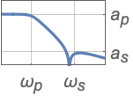
		{"Lowpass",{ω_p,ω_s},{a_p,a_s}}	パスバンドとストップバンドの周波数と減衰を使ったローパスフィルタ
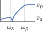
		{"Highpass",{ω_s,ω_p},{a_s,a_p}}	ハイパスフィルタ
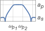
		{"Bandpass",{ω_s1,ω_p1,ω_p2,ω_s2},{a_s,a_p}}	バンドパスフィルタ
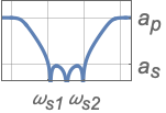
		{"Bandstop",{ω_p1,ω_s1,ω_s2,ω_p2},{a_p,a_s}}	バンドストップフィルタ

周波数値は昇順で与えられなければならない．
値 a_pと a_sはそれぞれパスバンドとストップバンドの減衰の絶対値である．
ゲインがのとき，減衰はである．

例題

すべて開くすべて閉じる

例 (2)

3次第2種チェビシェフフィルタモデル：

Wolfram Language code: tf = Chebyshev2FilterModel[3]

フィルタモデルを変数で表現する：

Wolfram Language code: tf = Chebyshev2FilterModel[3, s]

モデル化されたフィルタのボード線図：

Wolfram Language code: BodePlot[tf, GridLines -> Automatic, PlotLayout -> "Magnitude"]

完全指定を用いたローパス第2種チェビシェフフィルタ：

Wolfram Language code: tf = Chebyshev2FilterModel[{"Lowpass", {1., 2.}, {1., 20.}}, s]//Chop

理想的なフィルタ特性を示しているフィルタの大きさ応答：

Wolfram Language code:

Plot[Abs[tf[I * ω]], {ω, 0, 3}, PlotRange -> All, Epilog -> {Pink, Dashed, Line[{{0, 0.89}, {1, 0.89}, {1, 0.1}}], Line[{{2., 0.89}, {2., 0.1}, {3., 0.1}}]}]

スコープ (5)

2次ローパスフィルタの記号表現：

Wolfram Language code: Chebyshev2FilterModel[{2, ω}, s]//N//Chop

モデルの厳密計算：

Wolfram Language code: Chebyshev2FilterModel[{2, 1}, s]

24桁精度でのモデルの計算：

Wolfram Language code: Chebyshev2FilterModel[{2, N[1, 24]}, s]

ハイパスの第2種チェビシェフフィルタを作る：

Wolfram Language code: BodePlot[Chebyshev2FilterModel[{"Highpass", {1., 2.}, {20., 1.}}], GridLines -> Automatic, PlotLayout -> "Magnitude"]

バンドパス第2種チェビシェフフィルタを作る：

Wolfram Language code:

BodePlot[Chebyshev2FilterModel[{"Bandpass", {1., 10., 100., 1000.}, {20., 1.}}], GridLines -> Automatic, PlotLayout -> "Magnitude"]

バンドストップ第2種チェビシェフフィルタを作る：

Wolfram Language code:

BodePlot[Chebyshev2FilterModel[{"Bandstop", {1., 10., 100., 1000.}, {1, 20}}], GridLines -> Automatic, PlotLayout -> "Magnitude"]

アプリケーション (5)

ローパスの第2種チェビシェフフィルタを作る：

Wolfram Language code: tf = Chebyshev2FilterModel[{"Lowpass", {1., 2.}, {1, 40}}, s];

フィルタで正弦波信号から高周波ノイズを取り除く：

Wolfram Language code:

ω = 1 / 5;input = (Sin[ω t] + 1 / 2 Sin[25ω t]) UnitStep[t];
response1 = OutputResponse[tf, input, {t, 0, 100}];

第2種チェビシェフフィルタの位相は，Arg[tf[ω ]]による応答を移動させる．この場合，ω は入力正弦曲線の周波数である：

Wolfram Language code: Plot[{input, response1}, {t, 20, 100}]

位相のシフトを正す：

Wolfram Language code:

delay = Arg[tf[I ω]] / ω//First//First;
Plot[Evaluate[Flatten[{input, response1 /. t -> (t - delay)}]], {t, 20, 100}]

ローパスのプロトタイプからハイパスの第2種チェビシェフフィルタを作る：

Wolfram Language code: tf2 = TransferFunctionTransform[1 / #&, tf];

フィルタで入力から低周波正弦曲線を取り除く：

Wolfram Language code: Plot[Evaluate[Flatten[{input, OutputResponse[tf2, input, {t, 0, 100}]}]], {t, 20, 100}]

次のパスバンド周波数，ストップバンド周波数，減衰を満足する第2種チェビシェフ近似を使ってデジタルローパスフィルタを設計する：

Wolfram Language code:

Subscript[ω, p] = 0.4π;Subscript[ω, s] = 0.6π;
Subscript[a, p] = 1;Subscript[a, s] = 20;

サンプリング周期が1であると仮定して，同等のアナログ周波数を得る：

Wolfram Language code: {Subscript[Ω, p] = 2 Tan[(0.4π/2)], Subscript[Ω, s] = 2 Tan[(0.6π/2)]}

アナログ第1種チェビシェフ伝達関数を計算する：

Wolfram Language code: tf = Chebyshev2FilterModel[{"Lowpass", {Subscript[Ω, p], Subscript[Ω, s]}, {Subscript[a, p], Subscript[a, s]}}, s]

離散時間モデルに変換する：

Wolfram Language code: dtf = ToDiscreteTimeModel[tf, 1, z]//Chop

大きさをプロットする：

Wolfram Language code:

BodePlot[dtf, {0.1 π, π}, PlotLayout -> "Magnitude", GridLines -> {{Subscript[ω, p], Subscript[ω, s]}, {10^-Subscript[a, p] / 20, 10^-Subscript[a, s] / 20}}, ScalingFunctions -> {"Linear", "Absolute"}, PlotRange -> All]

離散時間第2種チェビシェフIIRフィルタの長さ21のFIR近似を作成する：

Wolfram Language code: OutputResponse[dtf, KroneckerDelta[n], {n, 0, 20}]//Chop

FIRフィルタをプロットする：

Wolfram Language code: ListPlot[%, PlotRange -> All, Filling -> 0]

チェビシェフフィルタのFIR近似を使って金融データを平滑化する：

Wolfram Language code:

data = Transpose[FinancialData["GE", {"Jan. 1, 2012", "Jan. 1, 2013"}]["Path"]];
fir = OutputResponse[ToDiscreteTimeModel[Chebyshev2FilterModel[{3, 0.5}], 1], KroneckerDelta[n], {n, 0, 40}]//Chop//Flatten;
DateListPlot[{Transpose[data], Transpose[{data[[1]], -ListConvolve[fir, data[[2]], 4]}]}, PlotRange -> All, PlotLegends -> {"original", "smoothed"}]

ローパスの第2種チェビシェフフィルタを使って画像にフィルタをかける：

Wolfram Language code:

h = ToDiscreteTimeModel[Chebyshev2FilterModel[3], 1];
RecurrenceFilter[h, [image]]

ハイパスの第2種チェビシェフフィルタを使って画像にフィルタをかける：

Wolfram Language code:

h = ToDiscreteTimeModel[Chebyshev2FilterModel[{"Highpass", {.5, 1}, {20, 1}}], 1];
RecurrenceFilter[h, [image]]

特性と関係 (5)

ローパスの第1種チェビシェフフィルタと第2種チェビシェフフィルタを比較する：

Wolfram Language code: t1 = Chebyshev1FilterModel[{"Lowpass", {1., 2.}, {1., 20.}}]

Wolfram Language code: t2 = Chebyshev2FilterModel[{"Lowpass", {1., 2.}, {1., 20.}}]

Wolfram Language code:

Plot[{Abs[t1[I * ω]], Abs[t2[I * ω]]}, {ω, 0, 3}, PlotRange -> All, Epilog -> {Pink, Dashed, Line[{{0, 0.89}, {1, 0.89}, {1, 0.1}}], Line[{{2., 0.89}, {2., 0.1}, {3., 0.1}}]}]

第2種多項式チェビシェフフィルタの次数を抽出する：

Wolfram Language code: SystemsModelOrder[StateSpaceModel[Chebyshev2FilterModel[{"Lowpass", {1., 2.}, {1., 20.}}]]]

第2種チェビシェフフィルタの極と零点を求める：

Wolfram Language code: tfm = Chebyshev2FilterModel[11];

Wolfram Language code: {poles, zeros} = Through[{TransferFunctionPoles, TransferFunctionZeros}[tfm]]

チェビシェフフィルタの極と零点をプロットする：

Wolfram Language code: PoleZeroPlot[tfm]

ローパスデジタル第2種チェビシェフフィルタを実装する：

Wolfram Language code: dtfm = ToDiscreteTimeModel[Chebyshev2FilterModel[11], 1]

デジタル第2種チェビシェフフィルタの極と零点をプロットする：

Wolfram Language code: PoleZeroPlot[dtfm]

ローパスフィルタをハイパスフィルタに変換する：

Wolfram Language code:

lo = Chebyshev2FilterModel[3];
hi = TransferFunctionTransform[(1 / #&), lo]

Wolfram Language code: Plot[{Abs[lo[I w]], Abs[hi[I w]]}, {w, 0, 3}, PlotRange -> All]

考えられる問題 (1)

記号フィルタは，次数が計算できないので，完全指定では返すことができない：

Wolfram Language code: Chebyshev2FilterModel[{"Lowpass", {ωp, ωs}, {ap, as}}]

Top

その他のラーニングリソース

テクニカルサポート

データサイエンス，金融，ビジネス

工学

科学とテクノロジー

教育のためのテクノロジー

教育イニシアチブ

使い始める

Grow Your Skills

Wolframと繋がる

大人用の教育プログラム

若者のための教育プログラム

読む

Chebyshev2FilterModel

詳細

例題

例 (2)

スコープ (5)

アプリケーション (5)

特性と関係 (5)

考えられる問題 (1)

テキスト

CMS

APA

BibTeX

BibLaTeX

Chebyshev2FilterModel

詳細

例題

例 (2)

スコープ (5)

アプリケーション (5)

特性と関係 (5)

考えられる問題 (1)

関連項目

関連するガイド

履歴

テキスト

CMS

APA

BibTeX

BibLaTeX