

给出图 g 的连通分量.
ConnectedComponents[g,{v1,v2,…}]
给出至少包括顶点 v1、v2、… 中的一个的连通分量.
ConnectedComponents[g,patt]
给出包含与模式 patt 匹配的顶点的连通分量.
ConnectedComponents[{vw,…},…]
使用规则 vw 来指定图 g.
ConnectedComponents
给出图 g 的连通分量.
ConnectedComponents[g,{v1,v2,…}]
给出至少包括顶点 v1、v2、… 中的一个的连通分量.
ConnectedComponents[g,patt]
给出包含与模式 patt 匹配的顶点的连通分量.
ConnectedComponents[{vw,…},…]
使用规则 vw 来指定图 g.
更多信息
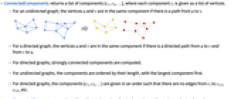
- ConnectedComponents 返回分量列表 {c1,c2,…},其中每个分量 ci 以顶点列表的形式给出.
- 对于一个无向图,如果存在从 u 到 v 的一条路径,则顶点 u 和 v 在同一个分量中.
- 对于一个有向图,如果存在从 u 到 v 和从 v 到 u 的有向路径,则称顶点 u 和 v 在同一个分量中.
- 对于有向图,计算强连通分量.
- 对于无向图,分量以它们的长度排序,其中最大的分量排在第一位.
- 对于有向图,分量 {c1,c2,…} 以这样的顺序给出:不存在从 ci,到 ci+1、ci+2 等的边.
- ConnectedComponents 适用于无向图、有向图、多重图和混合图.

范例
打开所有单元 关闭所有单元基本范例 (1)
范围 (8)
ConnectedComponents 适用于无向图:
ConnectedComponents[[image]]ConnectedComponents[[image]]ConnectedComponents[[image]]ConnectedComponents[[image]]ConnectedComponents[{3 -> 1, 1 -> 5, 2 -> 4, 2 -> 6, 3 -> 5, 4 -> 6}]ConnectedComponents[[image], {1, 7}]ConnectedComponents[[image], v_ ? EvenQ]ConnectedComponents 可用于大规模图:
RandomGraph[{10000, 20000}];ConnectedComponents[%]//Shallow//Timing应用 (4)
g = DirectedGraph[GridGraph[{10, 30}], "Random", VertexSize -> 0.6, GraphHighlightStyle -> "DehighlightFade"];HighlightGraph[g, Select[ConnectedComponents[g], Length[#] > 1&]]荷花池的一只青蛙能够跳1.5英尺,从25支荷叶中的一支跳到另外一支. 根据荷叶密度和 SpatialGraphDistribution 模拟青蛙的跳跃网络:
lilyDensity = MixtureDistribution[{1, 1, 1}, {BinormalDistribution[{0, 0}, {1, 1}, 0], BinormalDistribution[{-1, 4}, {1, 1}, -1 / 2], BinormalDistribution[{4, 4}, {1, 1}, 1 / 3]}];lilyPond = SpatialGraphDistribution[25, 1.5, lilyDensity];g = RandomGraph[lilyPond, VertexShape -> [image], VertexSize -> {"Scaled", 0.1}, EdgeStyle -> Opacity[0], Background -> Hue[0.6, 0.8, 0.4], ImageSize -> 150]Length[First[ConnectedComponents[g]]]largestIsland = GraphPropertyDistribution[Length[First[ConnectedComponents[g]]], glilyPond];RandomVariate[largestIsland, 10]Length[ConnectedComponents[g]] - 1frogSwims = GraphPropertyDistribution[Length[ConnectedComponents[g]] - 1, glilyPond];RandomVariate[frogSwims, 10]A = (| | | | | |
| -- | -- | -- | -- | -- |
| 0 | 0 | a2 | 0 | 0 |
| 0 | 0 | 0 | 0 | a3 |
| a5 | 0 | 0 | 0 | 0 |
| 0 | 0 | 0 | a4 | 0 |
| 0 | a1 | 0 | 0 | 0 |);AdjacencyGraph[Map[Boole[!PossibleZeroQ[#]]&, A, {2}]]ConnectedComponents[%]p = Flatten[%]A[[InversePermutation[p], p]]//MatrixForm属性和关系 (4)
使用 WeaklyConnectedComponents 来获取有向图的弱连通分量:
g = Graph[{12, 23, 31, 34, 45, 35, 67}]WeaklyConnectedComponents[g]ConnectedComponents[UndirectedGraph[g]]使用 ConnectedGraphQ 来测试一个图是否连通:
RandomGraph[{10, 8}]ConnectedGraphQ[%]g = GridGraph[{2, 3}]ConnectedGraphQ[g]ConnectedComponents[g]//Lengthg = RandomGraph[{10, 8}]Length[ConnectedComponents[g]] ≥ VertexCount[g] - EdgeCount[g]文本
Wolfram Research (2010),ConnectedComponents,Wolfram 语言函数,https://reference.wolfram.com/language/ref/ConnectedComponents.html (更新于 2015 年).
CMS
Wolfram 语言. 2010. "ConnectedComponents." Wolfram 语言与系统参考资料中心. Wolfram Research. 最新版本 2015. https://reference.wolfram.com/language/ref/ConnectedComponents.html.
APA
Wolfram 语言. (2010). ConnectedComponents. Wolfram 语言与系统参考资料中心. 追溯自 https://reference.wolfram.com/language/ref/ConnectedComponents.html 年
BibTeX
@misc{reference.wolfram_2026_connectedcomponents, author="Wolfram Research", title="{ConnectedComponents}", year="2015", howpublished="\url{https://reference.wolfram.com/language/ref/ConnectedComponents.html}", note=[Accessed: 14-September-2026]}
BibLaTeX
@online{reference.wolfram_2026_connectedcomponents, organization={Wolfram Research}, title={ConnectedComponents}, year={2015}, url={https://reference.wolfram.com/language/ref/ConnectedComponents.html}, note=[Accessed: 14-September-2026]}