

DiscreteMarkovProcess[i0,m]
遷移行列 m,初期状態 i0の離散時間有限状態のマルコフ(Markov)過程を表す.
DiscreteMarkovProcess[p0,m]
初期状態確率ベクトルが p0のマルコフ過程を表す.
グラフ g からの遷移行列を持つマルコフ過程を表す.
DiscreteMarkovProcess
DiscreteMarkovProcess[i0,m]
遷移行列 m,初期状態 i0の離散時間有限状態のマルコフ(Markov)過程を表す.
DiscreteMarkovProcess[p0,m]
初期状態確率ベクトルが p0のマルコフ過程を表す.
グラフ g からの遷移行列を持つマルコフ過程を表す.
詳細
- DiscreteMarkovProcessは離散時間マルコフ連鎖としても知られている.
- DiscreteMarkovProcessは離散時間・離散状態のランダム過程である.
- DiscreteMarkovProcessの状態は1から
までの整数である.ただし,
は遷移行列 m の長さである. - 遷移行列 m は条件付きの遷移確率 m〚i,j〛Probability[x[k+1]jx[k]i]を指定する.ただし,x[k]は時間 k における過程の状態である. »
- 離散マルコフ過程はグラフ上のランダムウォークと見ることができる.ただし,状態
から状態
への遷移確率は m〚i,j〛で指定される. - DiscreteMarkovProcess[n]は,EstimatedProcessおよび関連関数で使用するための,n 個の状態を持つ離散時間マルコフ過程を表す. »
- グラフ g の場合の遷移行列は,各接続頂点の遷移確率が等しくなるように構築される.
- DiscreteMarkovProcessでは,m は和が1になる非負の要素と行を持つ
×
行列,i0 は1から
までの整数,p0 は和が1になる非負の要素の長さ
のベクトルである. - DiscreteMarkovProcessは,MarkovProcessProperties,PDF,Probability,RandomFunction等の関数で使うことができる.
例題
すべて開く すべて閉じる例 (2)
𝒫 = DiscreteMarkovProcess[{1, 0, 0}, {{0, (1/2), (1/2)}, {(1/2), 0, (1/2)}, {(1/2), (1/2), 0}}];data = RandomFunction[𝒫, {0, 10}]ListPlot[data, Filling -> Axis, Ticks -> {Automatic, {1, 2, 3}}]𝒫 = DiscreteMarkovProcess[{1, 0, 0}, {{0, (1/2), (1/2)}, {(1/2), 0, (1/2)}, {(1/2), (1/2), 0}}];PDF[𝒫[n], k]//PiecewiseExpandPDF[StationaryDistribution[𝒫], 2]スコープ (15)
MarkovProcessProperties[DiscreteMarkovProcess[3, {{1 / 2, 1 / 2, 0, 0}, {1 / 2, 1 / 2, 0, 0}, {1 / 4, 1 / 4, 1 / 4, 1 / 4}, {0, 0, 0, 1}}]]遷移確率をツールチップで与え,過程をグラフとして可視化する:
Graph[DiscreteMarkovProcess[3, {{1 / 2, 1 / 2, 0, 0}, {1 / 2, 1 / 2, 0, 0}, {1 / 4, 1 / 4, 1 / 4, 1 / 4}, {0, 0, 0, 1}}]]DiscreteMarkovProcess[3, %]Mean[FirstPassageTimeDistribution[DiscreteMarkovProcess[1, {{0, (1/2), (1/2)}, {(1/2), 0, (1/2)}, {(1/2), (1/2), 0}}], 3]]StationaryDistribution[DiscreteMarkovProcess[1, {{1 - a, a}, {b, 1 - b}}]]DiscreteMarkovProcess[1, {{1 - a, a}, {b, 1 - b}}][Infinity]遷移行列がSparseArrayとして与えられる過程の定常分布:
tm = SparseArray[{{5, 1} -> 1, {i_, 1} -> 1 / 2, {i_, j_} /; j == i + 1 -> 1 / 2}, {5, 5}];StationaryDistribution[DiscreteMarkovProcess[1, tm]]𝒫 = DiscreteMarkovProcess[4, {{1, 0, 0, 0}, {0.1, 0.4, 0.2, 0.3}, {0, 0, 1, 0}, {0.4, 0, 0.2, 0.4}}];MarkovProcessProperties[𝒫, "AbsorbingClasses"]PDF[𝒫[∞], 1]𝒫 = DiscreteMarkovProcess[3, {{1 / 2, 1 / 2, 0, 0}, {1 / 2, 1 / 2, 0, 0}, {1 / 4, 1 / 4, 1 / 4, 1 / 4}, {0, 0, 0, 1}}];MarkovProcessProperties[𝒫, "CommunicatingClasses"]MarkovProcessProperties[𝒫, "RecurrentClasses"]MarkovProcessProperties[𝒫, "TransientClasses"]𝒫 = DiscreteMarkovProcess[3, {{1 / 2, 1 / 2, 0, 0}, {1 / 2, 1 / 2, 0, 0}, {1 / 4, 1 / 4, 1 / 4, 1 / 4}, {0, 0, 0, 1}}];BlockRandom[SeedRandom[1234];data = RandomFunction[𝒫, {0, 25}]]DiscretePlot[Evaluate[data["PathFunction"][t]], {t, data["MinimumTime"], data["MaximumTime"]}, ExtentSize -> 1, Ticks -> {Automatic, Range[Max[data["Values"]]]}]𝒫 = DiscreteMarkovProcess[3, {{1 / 2, 1 / 2, 0, 0}, {1 / 2, 1 / 2, 0, 0}, {1 / 4, 1 / 4, 1 / 4, 1 / 4}, {0, 0, 0, 1}}];data = RandomFunction[𝒫, {0, 10 ^ 3}, 10 ^ 2];Map[MatrixForm, EstimatedProcess[data, DiscreteMarkovProcess[4]]]対象状態への到達についての条件付きで最初の移行時間の平均と分散を求める:
𝒫 = DiscreteMarkovProcess[3, {{1 / 2, 1 / 2, 0, 0}, {1 / 2, 1 / 2, 0, 0}, {1 / 4, 1 / 4, 1 / 4, 1 / 4}, {0, 0, 0, 1}}];𝒟 = FirstPassageTimeDistribution[𝒫, {1, 2}];{Mean[𝒟], Variance[𝒟]}data = Select[Normal[RandomFunction[𝒫, {0, 10 ^ 4}, 10 ^ 4, Method -> {Automatic, "StoppingFunction" -> Function[{len, pos}, !MemberQ[{1, 2, 4}, pos]]}]], MemberQ[{1, 2}, #[[-1, -1]]]&];Comap[{Mean, Variance}, N[Length[#] - 1]& /@ data]proc = DiscreteMarkovProcess[{1 / 4, 3 / 4}, {{2 / 3, 1 / 3}, {1 / 3, 2 / 3}}];Probability[x[t] ^ 2 + x[t] < 6, xproc]//SimplifyN[% /. t -> 3]NProbability[x ^ 2 + x < 6, xproc[3]]proc = DiscreteMarkovProcess[{1 / 4, 3 / 4}, {{2 / 3, 1 / 3}, {1 / 3, 2 / 3}}];Probability[x[10] == 2 && x[60] - x[45] == 1, xproc]proc = DiscreteMarkovProcess[1, {{1 / 2, 1 / 2, 0, 0}, {1 / 2, 0, 1 / 6, 1 / 3}, {0, 0, 1, 0}, {0, 0, 0, 1}}];Probability[x[n] == 3x[n] > 2, xproc]//FullSimplify[#, Element[n, Integers] && n > 1]&Probability[x[n] == 4x[n] > 2, xproc]//FullSimplify[#, Element[n, Integers] && n > 1]&proc = DiscreteMarkovProcess[{1 / 4, 3 / 4}, {{2 / 3, 1 / 3}, {1 / 3, 2 / 3}}];Expectation[x + E ^ (-x), xproc[t]]//SimplifyN[% /. t -> 7]NExpectation[x + E ^ (-x), xproc[7]]proc = DiscreteMarkovProcess[{1 / 4, 3 / 4}, {{2 / 3, 1 / 3}, {1 / 3, 2 / 3}}];Moment[proc[t], r]CharacteristicFunction[proc[t], w]//SimplifyCentralMomentGeneratingFunction[proc[t], w]//Simplifyグラフ表現で賭博者の破滅過程のシミュレーションを可視化する:
GamblersRuin[p_, n_] := SparseArray[{{1, 1} -> 1, {n + 1, n + 1} -> 1, {i_, j_} /; 1 < i < n + 1 && j == i + 1 -> p, {i_, j_} /; 1 < i < n + 1 && j == i - 1 -> 1 - p}, {n + 1, n + 1}]gamblerwealth = DiscreteMarkovProcess[4, GamblersRuin[0.4, 7]];BlockRandom[SeedRandom[12360];path = RandomFunction[gamblerwealth, {0, 35}]["Values"]]Manipulate[Graph[gamblerwealth, GraphHighlight -> path[[time + 1]], GraphHighlightStyle -> "VertexConcaveDiamond", PlotLabel -> "Time = " <> ToString[time], ImageSize -> Medium], {time, 0, Length[path] - 1, 1}, SaveDefinitions -> True]一般化と拡張 (2)
gr = Graph[{12, 21, 22}, AnnotationRules -> {1 -> {"InitialProbability" -> 0.6}, 2 -> {"InitialProbability" -> 0.4}, 12 -> {"Probability" -> 1}, 21 -> {"Probability" -> 1 / 3}, 22 -> {"Probability" -> 2 / 3}}];DiscreteMarkovProcess[gr]//Normal類を別々の色を使ってハイライトし,離散マルコフ過程をグラフとして表す:
proc = DiscreteMarkovProcess[1, {{(1/2), (1/2), 0, 0, 0}, {(1/3), (2/3), 0, 0, 0}, {0, (1/3), (2/3), 0, 0}, {0, 0, 0, 0, 1}, {0, 0, 0, 1, 0}}];Graph[proc]アプリケーション (18)
ゲーム (7)
繰り返しコインを投げ上げる過程を,表が出る確率が0.6で裏が出る過程が0.4の離散マルコフ過程を使ってモデル化する:
coin = DiscreteMarkovProcess[1, {{0.6, 0.4}, {0.6, 0.4}}];tosses = RandomFunction[coin, {0, 49}]ListPlot[tosses, Ticks -> {Automatic, {{1, "Head"}, {2, "Tail"}}}, Filling -> Axis]表が出る確率が
の不正なコインを
回はじく.連続して表が出続ける最高回数が指定の数
を超える確率を求める.これは,状態
が
回連続して表が出たことを表す離散マルコフ過程を使ってモデル化することができる.結果の,
,
,
の遷移行列は以下で与えられる:
m = With[{p = 0.6, k = 10}, SparseArray[{Band[{1, 2}] -> p, {i_, 1} /; i ≤ k -> 1 - p, {k + 1, k + 1} -> 1}]];
MatrixForm[m]連続して表が出る回数のシミュレーションを行う.表が連続して10回出た場合は再び数え始めないこととする:
SeedRandom[8];
heads = RandomFunction[DiscreteMarkovProcess[1, m], {0, 200}];ListLinePlot[heads, Ticks -> {Automatic, Table[If[i < 11, {i, i - 1}, {i, ">= 10"}], {i, 11}]}, PlotRange -> {1, 11}]100回コインをはじいた場合に最低でも10回連続して表が出る確率:
Probability[x[100] == 11, xDiscreteMarkovProcess[1, m]]ある賭博師が3つのチップから始めて,勝つ確率が0.4で,無一文になる前にチップ7つ勝つことを目標にして,各ステップで1チップの賭けを行う.ここで状態は,整数1から8で,賭博師の富に1足したものを表す:
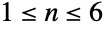
GamblersRuin[p_, n_] := SparseArray[{{1, 1} -> 1, {n + 1, n + 1} -> 1, {i_, j_} /; 1 < i < n + 1 && j == i + 1 -> p, {i_, j_} /; 1 < i < n + 1 && j == i - 1 -> 1 - p}, {n + 1, n + 1}]gamblerwealth = DiscreteMarkovProcess[4, GamblersRuin[0.4, 7]];SeedRandom[2345];ListLinePlot[{#[[1]], #[[2]] - 1}& /@ RandomFunction[gamblerwealth, {0, 30}]["Path"], InterpolationOrder -> 0]Transpose[{MarkovProcessProperties[gamblerwealth, "TransientClasses"][[1]] - 1, MarkovProcessProperties[gamblerwealth, "TransientVisitMean"]}]//TableFormdata = RandomFunction[gamblerwealth, {0, 10 ^ 3}, 10 ^ 4, Method -> {Automatic, "StoppingFunction" -> Function[{len, pos}, len < 1001 && pos ≠ 1 && pos ≠ 8]}]["ValueList"];Table[Mean[Count[#, i]& /@ data], {i, 2, 7}]//N賭博師が目標を達成する,あるいは無一文になるまでの期待時間を求める:
Mean[FirstPassageTimeDistribution[gamblerwealth, {1, 8}]]賭博師が目標を達成する,あるいは無一文になるまでに訪問する状態の合計:
MarkovProcessProperties[gamblerwealth, "TransientTotalVisitMean"]data = DeleteDuplicates /@ RandomFunction[gamblerwealth, {0, 10 ^ 2}, 4 * 10 ^ 3]["ValueList"];Mean[Length[#] - 1& /@ data]//NPDF[gamblerwealth[Infinity], 8]サイコロの6面すべてが出るまでに平均で何回サイコロを振らなければならないかを求める:
dierolls = DiscreteMarkovProcess[1, With[{numfaces = 6}, SparseArray[{{i_, i_} -> (i - 1) / numfaces, {i_, j_} /; (j - i - 1 == 0) -> (numfaces - (i - 1)) / numfaces}, {numfaces + 1, numfaces + 1}]]];Mean[FirstPassageTimeDistribution[dierolls, 7]]probs = Refine[Probability[x[n] == 7, xdierolls], n > 0]ListPlot[Table[probs, {n, 1, 6 * 6}]]公正なコインをはじいたときに,その結果が裏表表の順となるマルコフ過程:
proc1 = DiscreteMarkovProcess[1, {{1 / 2, 1 / 2, 0, 0}, {0, 1 / 2, 1 / 2, 0}, {0, 1 / 2, 0, 1 / 2}, {0, 0, 0, 1}}];Graph[proc1]公正なコインをはじいたときに,その結果が表表表の順となるマルコフ過程:
proc2 = DiscreteMarkovProcess[1, {{1 / 2, 1 / 2, 0, 0}, {1 / 2, 0, 1 / 2, 0}, {1 / 2, 0, 0, 1 / 2}, {0, 0, 0, 1}}];Graph[proc2]FirstPassageTimeDistribution[proc1, 4]//MeanFirstPassageTimeDistribution[proc2, 4]//Mean2人の選手間のテニスの試合で,サーブする人がポイントを得る確率が
であると仮定する.可能な状態は全部で17である:
states = {"GameA", "GameB", "Deux", "AdvA", "AdvB", "40-15", "15-40", "40-0", "30-15", "15-30", "0-40", "30-0", "15-15", "0-30", "15-0", "0-15", "0-0"};proc = With[{p = 3 / 5, q = 2 / 5}, DiscreteMarkovProcess[17, SparseArray[{{1, 1} -> 1, {2, 2} -> 1, {3, 4} -> p, {3, 5} -> q, {4, 1} -> p, {4, 3} -> q, {5, 2} -> q, {5, 3} -> p, {6, 1} -> p, {6, 4} -> q, {7, 2} -> q, {7, 5} -> p, {8, 1} -> p, {8, 6} -> q, {9, 3} -> q, {9, 6} -> p, {10, 3} -> p, {10, 7} -> q, {11, 2} -> q, {11, 7} -> p, {12, 8} -> p, {12, 9} -> q, {13, 9} -> p, {13, 10} -> q, {14, 10} -> p, {14, 11} -> q, {15, 12} -> p, {15, 13} -> q, {16, 13} -> p, {16, 14} -> q, {17, 15} -> p, {17, 16} -> q}, {17, 17}]]];Graph[proc, VertexSize -> Large, VertexLabels -> Thread[Range[17] -> Map[Placed[Style[#, {Bold}], Center]&, states]], ImageSize -> Large, ImagePadding -> 25]PDF[proc[Infinity], 1]//NMarkovProcessProperties[proc, "ReachabilityProbability"][[1]]//NN[Mean[FirstPassageTimeDistribution[proc, {1, 2}]]]Total[MarkovProcessProperties[proc, "TransientVisitMean"]]//NMarkovProcessProperties[proc, "TransientTotalVisitMean"]//NMarkovProcessProperties[proc, "TransientVisitMean"][[1]]//NMean[Count[#, 3]& /@ RandomFunction[proc, {0, 10 ^ 3}, 10 ^ 4, Method -> {Automatic, "StoppingFunction" -> Function[{len, pos}, len < 1001 && pos ≠ 1 && pos ≠ 2]}]["ValueList"]]//Nクラップスのゲームでは,2つのサイコロを投げてその出た目の数を合計する.第1投では,7か11が出ると勝ち,2か3か12が出ると負けで,それ以外の数が出た場合にはポイントとなり,サイコロが投げ続けられる.その後は,投げ手がポイントを出すと勝ちで,7が出ると負けである.状態は,開始,勝ち,負け,p4,p5,p6,p8,p9,p10のいずれかである.最初に戻ることは決してないが,勝ちと負けは吸収状態である.以下の分布は2つのサイコロを投げた場合を表す:
len = Length[Flatten[Map[Permutations, IntegerPartitions[#, {2}, Range[6]]], 1]]& /@ Range[2, 12];dist = ProbabilityDistribution[(len / Total[len]).Map[Boole[k == #]&, Range[2, 12]], {k, 1, 12, 1}];probwin = Probability[x == 7 || x == 11, xdist]problose = Probability[x == 2 || x == 3 || x == 12, xdist]第1投でその他の数が出ると,「ポイント」となり,投げ続ける:
probpoint = Probability[x == #, xdist]& /@ {4, 5, 6, 8, 9, 10}problose2 = Probability[x == 7, xdist]probstay = 1 - probpoint - problose2(m = Join[{Join[{0, probwin, problose}, probpoint], UnitVector[9, 2], UnitVector[9, 3]}, Transpose[Join[{ConstantArray[0, Length[probpoint]], probpoint, ConstantArray[problose2, Length[probpoint]]}, DiagonalMatrix[1 - probpoint - problose2]]]])//N//MatrixFormPDF[DiscreteMarkovProcess[1, m][Infinity], {2, 3}]N[%]Mean[FirstPassageTimeDistribution[DiscreteMarkovProcess[1, m], {2, 3}]]N[%]天候 (3)
単純な天候モデル:今日雨が降った場合,明日は確率0.7で雨が降る.今日雨が降らなければ,確率0.4で明日雨が降る.今日雨が降っているとした場合に,離散マルコフ過程を使ってこのモデルを表し,今日から4日後に雨が降る確率を求める.この天候の表現:
weather = DiscreteMarkovProcess[1, {{0.7, 0.3}, {0.4, 0.6}}];Graph[weather, VertexLabels -> {1 -> "rain", 2 -> "no rain"}, VertexSize -> Small, EdgeLabels -> With[{sm = MarkovProcessProperties[weather, "TransitionMatrix"]}, Flatten@Table[DirectedEdge[i, j] -> sm[[i, j]], {i, 2}, {j, 2}]], ImageSize -> Medium]Probability[rain[4] == 1, rainweather]過去2日間雨が降ったかどうかに基づいて天候のモデルを構築する.昨日と今日雨が降った場合は確率0.7で,今日は雨が降ったが昨日は雨が降らなかった場合は確率0.5で,昨日は雨が降ったが今日は降らなかった場合は確率0.4で,昨日も今日も雨が降らなかった場合は確率0.2で,明日雨が降るとする.積状態空間
を使う.ただし,
は昨日雨が降ったかどうかを,
は今日雨が降ったかどうかを示す:
rain[{"R", "R"}, {"R", "R"}] = 0.7;
rain[{"R", "R"}, {"R", "N"}] = 1 - 0.7;
rain[{"N", "R"}, {"R", "R"}] = 0.5;
rain[{"N", "R"}, {"R", "N"}] = 1 - 0.5;
rain[{"R", "N"}, {"N", "R"}] = 0.4;
rain[{"R", "N"}, {"N", "N"}] = 1 - 0.4;
rain[{"N", "N"}, {"N", "R"}] = 0.2;
rain[{"N", "N"}, {"N", "N"}] = 1 - 0.2;rain[s_, ns_] := 0m = ArrayFlatten@Table[rain[{x, y}, {z, w}], {x, {"R", "N"}}, {y, {"R", "N"}}, {z, {"R", "N"}}, {w, {"R", "N"}}]TableForm[m, TableHeadings -> {StringJoin /@ Tuples[{"R", "N"}, 2], StringJoin /@ Tuples[{"R", "N"}, 2]}]weather = DiscreteMarkovProcess[1, m];Evaluate[Map[state, StringJoin /@ Tuples[{"R", "N"}, 2]]] = Range[4];Probability[rain[4] == state["RR"] || rain[4] == state["NR"], rainweather]longtermWeather = StationaryDistribution[weather]Probability[rain == state["RR"], rainlongtermWeather]Count[RandomFunction[weather, {1, 10 ^ 4}]["Values"], 1] / 10 ^ 4//N空港か市内のどちらかにタクシーがいる.市内から次に空港へ行く確率は1/4,市内の別の場所へ行く確率は3/4である.空港からは常に市内へ戻る.状態1が市内を,状態2が空港を表す離散マルコフ過程を使って,空港から始めてタクシーをモデル化する:
taxi = DiscreteMarkovProcess[2, {{3 / 4, 1 / 4}, {1, 0}}];RandomFunction[taxi, {0, 20}]ListPlot[%, Ticks -> {Automatic, {{1, "City"}, {2, "Airport"}}}, Filling -> Axis]dist = StationaryDistribution[taxi]定常分布は,タクシーが営業時間の
を市内で過ごすことを示している:
DiscretePlot[PDF[dist, x], {x, {1, 2}}, ExtentSize -> Full, PlotRange -> {{0.5, 2.5}, {0, 1}}, Ticks -> {{1, 2}, Automatic}]壷 (1)
個のボールが壷Aと壷Bに分布している.各段階で1個のボールを無作為に選び,もう一方の壷に移す.壷Aのボールの定常分布を求める.壷Aに入っているボールの個数は離散マルコフ過程でモデル化することができる.壷Aに
個のボールが入っている場合,Aのボールを失う確率は
で,ボールを獲得する確率は
である.これは,遷移行列を与える:
(m = With[{n = 10}, Table[Which[j == i - 1, i / n, j == i + 1, 1 - i / n, True, 0], {i, 0, n}, {j, 0, n}]])StationaryDistribution[DiscreteMarkovProcess[1, m]]DiscretePlot[PDF[%, k], {k, 1, 11}, ExtentSize -> 1 / 2]SameQ@@Table[StationaryDistribution[DiscreteMarkovProcess[k, m]], {k, 1, 11}]ランダムウォーク (2)
両側で吸収するレイジーではないランダムウォークで,右に移動する可能性が2:1の場合,過程が左の境界の右横から始まったとしても,右の境界に到達する可能性は50%を超える:
PDF[DiscreteMarkovProcess[2, With[{n = 10}, SparseArray[{{1, 1} -> 1, {n, n} -> 1, Band[{2, 1}, {n - 1, n - 2}] -> 1 / 3, Band[{2, 3}] -> 2 / 3}, {n, n}]]][Infinity], {1, 10}]proc = DiscreteMarkovProcess[1, RotateRight[{1 / 3, 1 / 3, 0, 0, 0, 1 / 3},
#] & /@ Range[0, 5]];Graph[proc]MarkovProcessProperties[proc, "Reversible"]MarkovProcessProperties[proc, "Aperiodic"]StationaryDistribution[proc]機械修理 (1)
ある機械工場の作業セルは3台の機械からなっている.どの日でも機械のどれかが確率0.1で故障する.機械1は機械2と機械3の両方にフィードするので,機械1が故障するとその日は生産ができない.翌日使えるように同日修理できる機械は1台だけである.数台の機械が故障した場合,それらは1,2,3の優先順位で修理される.修理された機械は翌日は使えるものと仮定する.いくらかでも生産できる時間の割合を求める.故障と修理の過程は,故障している機械と使える機械のすべての組合せを列挙することで離散マルコフ過程としてモデル化することができる:
failed = Subsets[{1, 2, 3}]故障している機械がない.1台あるいは複数の機械が翌日故障する可能性がある:
transition[i_, j_] /; Length[i] == 0 := p^Length[j](1 - p)^3 - Length[j]1台の機械が故障している.これは修理される.残りの機械の片方あるいは両方が故障する可能性がある:
transition[i_, j_] /; Length[i] == 1 := p ^ Length[j](1 - p) ^ (3 - Length[j] - 1)Boole[Unequal@@Join[j, i]]2台の機械が故障している.修理は優先順位で行われる.残っている機械が故障する可能性がある:
transition[i_, j_] /; Length[i] == 2 && Length[j] == 1 := (1 - p)Boole[Rest[i] == j]transition[i_, j_] /; Length[i] == 2 && Length[j] == 2 := p Boole[And@@Thread[First[i] ≠ j]]transition[i_, j_] /; Length[i] == 2 := 0transition[i_, j_] /; Length[i] == 3 := Boole[j == {2, 3}](m = Block[{p = 0.1}, Table[transition[i, j], {i, failed}, {j, failed}]])//MatrixFormすべての機械が故障していない状態から始める離散マルコフ過程:
𝒫 = DiscreteMarkovProcess[1, m];Graph[𝒫, GraphLayout -> "BalloonEmbedding"]機械が1台も故障していない,あるいは機械2と3のどちらかだけが故障している場合に生産が行える:
Position[failed, {} | {2} | {3}]Probability[x == 1 || x == 3 || x == 4, xStationaryDistribution[𝒫]]Probability[x == 1, xStationaryDistribution[𝒫]]すべての機械が故障している状態から,1台も故障していない状態になるのにかかる時間の平均:
FirstPassageTimeDistribution[DiscreteMarkovProcess[8, m], 1]//Mean保険 (1)
Bonus–Malus自動車保険システムの4つの状態のマルコフ連鎖モデルで,それぞれの保険契約者は,その前の年に行った支払請求の数によって,1,2,3,4の状態のいずれかを与えられ,この状態が年払い保険料を決定する.支払請求がなければ,保険料が低くなるが,1回以上支払請求を行うと,通常保険料は高くなる.4つの状態について保険料のレベル
と,保険契約者の一連の状態の遷移行列を考慮して,保険契約者の年間の支払請求が平均
のポアソンランダム変数である場合の,年間保険料の平均を求める:
policyholderstates = DiscreteMarkovProcess[1, {{a[0], a[1], a[2], 1 - a[0] - a[1] - a[2]}, {a[0], 0, a[1], 1 - a[0] - a[1]}, {0, a[0], 0, 1 - a[0]}, {0, 0, a[0], 1 - a[0]}} /. a[k_] -> PDF[PoissonDistribution[1 / 2], k]]{200, 250, 400, 600}.PDF[StationaryDistribution[policyholderstates], Range[4]]//Nその他 (3)
1年が365日であり,どの日も等しい確率で誕生日に当ると仮定して,少なくとも2人が50%の確率で同じ誕生日となるには最低何人が必要かを求める.状態は,
— 誕生日が他の人と異なる人の数
および
— 少なくとも2人の人が同じ誕生日である:
proc = With[{n = 365}, DiscreteMarkovProcess[1, SparseArray[{{n, n + 1} -> 1, {n + 1, n + 1} -> 1, {i_, j_} /; j == i + 1 -> 1 - (i - 1) / n, {i_, n + 1} -> (i - 1) / n}, {n + 1, n + 1}]]];Position[With[{n = 365}, Table[PDF[proc[k], n + 1], {k, 1, 23}]], _ ? (# > 1 / 2&)]//Min孤島における種の個体数が食糧供給によって
で固定されている,簡単な自然淘汰のモデルを考慮する.突然変異体は,その種の通常の成員よりも高い生存率を生まれながらに持ち,それぞれの世代において,この突然変異体が確率
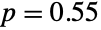
で位置を獲得するか,確率
で失う:
proc = DiscreteMarkovProcess[2, With[{n = 100}, SparseArray[{{1, 1} -> 1, {n, n} -> 1, Band[{2, 1}, {n - 1, n - 2}] -> 45 / 100, Band[{2, 3}] -> 55 / 100}, {n, n}]]];Probability[nmutants == 100, nmutantsproc[Infinity]]//NMean[FirstPassageTimeDistribution[proc, 100]]//N火星からの無線信号がたった1つの母音Aと4つの子音BCDRのみを使う言語で書かれており,通常の信号の中に次の推定遷移行列を持つマルコフ連鎖によって作成された長いメッセージがちりばめられていると仮定する:

sm = {{0, 1 / 2, 1 / 2, 0, 0}, {0, 1 / 3, 0, 1 / 3, 1 / 3}, {0, 0, 1 / 3, 1 / 3, 1 / 3}, {1 / 2, 0, 0, 0, 1 / 2}, {1 / 2, 0, 0, 0, 1 / 2}};proc = DiscreteMarkovProcess[1, sm];1 / PDF[StationaryDistribution[proc], 1]1 / (1 - PDF[StationaryDistribution[proc], 1]){Mean[#], Variance[#]}&[Length /@ DeleteCases[Split[RandomFunction[proc, {0, 10 ^ 5}]["Values"]], {1..} | {3..} | {4..} | {5..}]]N[%]{Mean[#], Variance[#]}&[TransformedDistribution[x + 1, xGeometricDistribution[1 - sm[[2, 2]]]]]N[%]特性と関係 (1)
考えられる問題 (3)
遷移行列の行を合計しても1にならない場合には,これらの行は正規化される:
DiscreteMarkovProcess[1, {{1, 2}, {4, 3}}]DiscreteMarkovProcess[{1, 2}, {{1 / 2, 1 / 2}, {2 / 3, 1 / 3}}]proc = DiscreteMarkovProcess[1, {{(1/2), (1/2), 0, 0, 0}, {(1/3), (2/3), 0, 0, 0}, {0, (1/3), (2/3), 0, 0}, {0, 0, 0, 0, 1}, {0, 0, 0, 1, 0}}];proc[Infinity]MarkovProcessProperties[proc, "Irreducible"]StationaryDistribution[DiscreteMarkovProcess[1, {{(1/2), (1/2), 0, 0, 0}, {(1/3), (2/3), 0, 0, 0}, {0, (1/3), (2/3), 0, 0}, {0, 0, 0, 0, 1}, {0, 0, 0, 1, 0}}]]StationaryDistribution[DiscreteMarkovProcess[4, {{(1/2), (1/2), 0, 0, 0}, {(1/3), (2/3), 0, 0, 0}, {0, (1/3), (2/3), 0, 0}, {0, 0, 0, 0, 1}, {0, 0, 0, 1, 0}}]]関連するガイド
-
▪
- 有限マルコフ(Markov)過程 ▪
- 有限数学 ▪
- 確率過程
テキスト
Wolfram Research (2012), DiscreteMarkovProcess, Wolfram言語関数, https://reference.wolfram.com/language/ref/DiscreteMarkovProcess.html (2014年に更新).
CMS
Wolfram Language. 2012. "DiscreteMarkovProcess." Wolfram Language & System Documentation Center. Wolfram Research. Last Modified 2014. https://reference.wolfram.com/language/ref/DiscreteMarkovProcess.html.
APA
Wolfram Language. (2012). DiscreteMarkovProcess. Wolfram Language & System Documentation Center. Retrieved from https://reference.wolfram.com/language/ref/DiscreteMarkovProcess.html
BibTeX
@misc{reference.wolfram_2026_discretemarkovprocess, author="Wolfram Research", title="{DiscreteMarkovProcess}", year="2014", howpublished="\url{https://reference.wolfram.com/language/ref/DiscreteMarkovProcess.html}", note=[Accessed: 15-September-2026]}
BibLaTeX
@online{reference.wolfram_2026_discretemarkovprocess, organization={Wolfram Research}, title={DiscreteMarkovProcess}, year={2014}, url={https://reference.wolfram.com/language/ref/DiscreteMarkovProcess.html}, note=[Accessed: 15-September-2026]}

