DiscreteMarkovProcess[i0,m]
表示转移矩阵为 m 和初始状态为 i0 的离散时间有限状态马可夫过程.
DiscreteMarkovProcess[p0,m]
表示初始状态概率向量为 p0 的马可夫过程.
表示来自图 g 的转移矩阵的马可夫链.
DiscreteMarkovProcess
DiscreteMarkovProcess[i0,m]
表示转移矩阵为 m 和初始状态为 i0 的离散时间有限状态马可夫过程.
DiscreteMarkovProcess[p0,m]
表示初始状态概率向量为 p0 的马可夫过程.
表示来自图 g 的转移矩阵的马可夫链.
更多信息
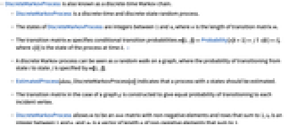
- DiscreteMarkovProcess 也称为离散时间马可夫链.
- DiscreteMarkovProcess 是一个离散时间和离散状态随机过程.
- DiscreteMarkovProcess 的状态是位于 1 和
之间的整数,其中
是转移矩阵 m 的长度. - 转移矩阵 m 指定了条件转移概率 m〚i,j〛Probability[x[k+1]jx[k]i],其中 x[k] 是时间 k 处过程的状态. »
- 离散马可夫过程可以被视为图上的随机游走,其中从状态
到状态
转移的概率由 m〚i,j〛 指定. - DiscreteMarkovProcess[n] 表示用于 EstimatedProcess 及相关函数的 n 状态离散时间马尔可夫过程. »
- 在图 g 中构建转移矩阵用来给出以相等概率转移至每个关联顶点.
- DiscreteMarkovProcess 中,m 是具有非负元素的
×
矩阵,其中各行之和为1,i0 是位于 1 和
之间的整数,而 p0 是由和为 1 的非负元素组成的长度为
的向量. - DiscreteMarkovProcess 可以与诸如 MarkovProcessProperties、PDF、Probability 和 RandomFunction 等函数一起使用.
范例
打开所有单元 关闭所有单元基本范例 (2)
𝒫 = DiscreteMarkovProcess[{1, 0, 0}, {{0, (1/2), (1/2)}, {(1/2), 0, (1/2)}, {(1/2), (1/2), 0}}];data = RandomFunction[𝒫, {0, 10}]ListPlot[data, Filling -> Axis, Ticks -> {Automatic, {1, 2, 3}}]𝒫 = DiscreteMarkovProcess[{1, 0, 0}, {{0, (1/2), (1/2)}, {(1/2), 0, (1/2)}, {(1/2), (1/2), 0}}];PDF[𝒫[n], k]//PiecewiseExpandPDF[StationaryDistribution[𝒫], 2]范围 (15)
MarkovProcessProperties[DiscreteMarkovProcess[3, {{1 / 2, 1 / 2, 0, 0}, {1 / 2, 1 / 2, 0, 0}, {1 / 4, 1 / 4, 1 / 4, 1 / 4}, {0, 0, 0, 1}}]]Graph[DiscreteMarkovProcess[3, {{1 / 2, 1 / 2, 0, 0}, {1 / 2, 1 / 2, 0, 0}, {1 / 4, 1 / 4, 1 / 4, 1 / 4}, {0, 0, 0, 1}}]]DiscreteMarkovProcess[3, %]Mean[FirstPassageTimeDistribution[DiscreteMarkovProcess[1, {{0, (1/2), (1/2)}, {(1/2), 0, (1/2)}, {(1/2), (1/2), 0}}], 3]]StationaryDistribution[DiscreteMarkovProcess[1, {{1 - a, a}, {b, 1 - b}}]]DiscreteMarkovProcess[1, {{1 - a, a}, {b, 1 - b}}][Infinity]对于转移矩阵由 SparseArray 给出的过程程,其平稳分布为:
tm = SparseArray[{{5, 1} -> 1, {i_, 1} -> 1 / 2, {i_, j_} /; j == i + 1 -> 1 / 2}, {5, 5}];StationaryDistribution[DiscreteMarkovProcess[1, tm]]𝒫 = DiscreteMarkovProcess[4, {{1, 0, 0, 0}, {0.1, 0.4, 0.2, 0.3}, {0, 0, 1, 0}, {0.4, 0, 0.2, 0.4}}];MarkovProcessProperties[𝒫, "AbsorbingClasses"]PDF[𝒫[∞], 1]𝒫 = DiscreteMarkovProcess[3, {{1 / 2, 1 / 2, 0, 0}, {1 / 2, 1 / 2, 0, 0}, {1 / 4, 1 / 4, 1 / 4, 1 / 4}, {0, 0, 0, 1}}];MarkovProcessProperties[𝒫, "CommunicatingClasses"]MarkovProcessProperties[𝒫, "RecurrentClasses"]MarkovProcessProperties[𝒫, "TransientClasses"]𝒫 = DiscreteMarkovProcess[3, {{1 / 2, 1 / 2, 0, 0}, {1 / 2, 1 / 2, 0, 0}, {1 / 4, 1 / 4, 1 / 4, 1 / 4}, {0, 0, 0, 1}}];BlockRandom[SeedRandom[1234];data = RandomFunction[𝒫, {0, 25}]]DiscretePlot[Evaluate[data["PathFunction"][t]], {t, data["MinimumTime"], data["MaximumTime"]}, ExtentSize -> 1, Ticks -> {Automatic, Range[Max[data["Values"]]]}]𝒫 = DiscreteMarkovProcess[3, {{1 / 2, 1 / 2, 0, 0}, {1 / 2, 1 / 2, 0, 0}, {1 / 4, 1 / 4, 1 / 4, 1 / 4}, {0, 0, 0, 1}}];data = RandomFunction[𝒫, {0, 10 ^ 3}, 10 ^ 2];Map[MatrixForm, EstimatedProcess[data, DiscreteMarkovProcess[4]]]𝒫 = DiscreteMarkovProcess[3, {{1 / 2, 1 / 2, 0, 0}, {1 / 2, 1 / 2, 0, 0}, {1 / 4, 1 / 4, 1 / 4, 1 / 4}, {0, 0, 0, 1}}];𝒟 = FirstPassageTimeDistribution[𝒫, {1, 2}];{Mean[𝒟], Variance[𝒟]}data = Select[Normal[RandomFunction[𝒫, {0, 10 ^ 4}, 10 ^ 4, Method -> {Automatic, "StoppingFunction" -> Function[{len, pos}, !MemberQ[{1, 2, 4}, pos]]}]], MemberQ[{1, 2}, #[[-1, -1]]]&];Comap[{Mean, Variance}, N[Length[#] - 1]& /@ data]proc = DiscreteMarkovProcess[{1 / 4, 3 / 4}, {{2 / 3, 1 / 3}, {1 / 3, 2 / 3}}];Probability[x[t] ^ 2 + x[t] < 6, xproc]//SimplifyN[% /. t -> 3]NProbability[x ^ 2 + x < 6, xproc[3]]proc = DiscreteMarkovProcess[{1 / 4, 3 / 4}, {{2 / 3, 1 / 3}, {1 / 3, 2 / 3}}];Probability[x[10] == 2 && x[60] - x[45] == 1, xproc]proc = DiscreteMarkovProcess[1, {{1 / 2, 1 / 2, 0, 0}, {1 / 2, 0, 1 / 6, 1 / 3}, {0, 0, 1, 0}, {0, 0, 0, 1}}];Probability[x[n] == 3x[n] > 2, xproc]//FullSimplify[#, Element[n, Integers] && n > 1]&Probability[x[n] == 4x[n] > 2, xproc]//FullSimplify[#, Element[n, Integers] && n > 1]&proc = DiscreteMarkovProcess[{1 / 4, 3 / 4}, {{2 / 3, 1 / 3}, {1 / 3, 2 / 3}}];Expectation[x + E ^ (-x), xproc[t]]//SimplifyN[% /. t -> 7]NExpectation[x + E ^ (-x), xproc[7]]proc = DiscreteMarkovProcess[{1 / 4, 3 / 4}, {{2 / 3, 1 / 3}, {1 / 3, 2 / 3}}];Moment[proc[t], r]CharacteristicFunction[proc[t], w]//SimplifyCentralMomentGeneratingFunction[proc[t], w]//SimplifyGamblersRuin[p_, n_] := SparseArray[{{1, 1} -> 1, {n + 1, n + 1} -> 1, {i_, j_} /; 1 < i < n + 1 && j == i + 1 -> p, {i_, j_} /; 1 < i < n + 1 && j == i - 1 -> 1 - p}, {n + 1, n + 1}]gamblerwealth = DiscreteMarkovProcess[4, GamblersRuin[0.4, 7]];BlockRandom[SeedRandom[12360];path = RandomFunction[gamblerwealth, {0, 35}]["Values"]]Manipulate[Graph[gamblerwealth, GraphHighlight -> path[[time + 1]], GraphHighlightStyle -> "VertexConcaveDiamond", PlotLabel -> "Time = " <> ToString[time], ImageSize -> Medium], {time, 0, Length[path] - 1, 1}, SaveDefinitions -> True]推广和延伸 (2)
gr = Graph[{12, 21, 22}, AnnotationRules -> {1 -> {"InitialProbability" -> 0.6}, 2 -> {"InitialProbability" -> 0.4}, 12 -> {"Probability" -> 1}, 21 -> {"Probability" -> 1 / 3}, 22 -> {"Probability" -> 2 / 3}}];DiscreteMarkovProcess[gr]//Normalproc = DiscreteMarkovProcess[1, {{(1/2), (1/2), 0, 0, 0}, {(1/3), (2/3), 0, 0, 0}, {0, (1/3), (2/3), 0, 0}, {0, 0, 0, 0, 1}, {0, 0, 0, 1, 0}}];Graph[proc]应用 (18)
游戏 (7)
对重复投掷一个硬币的过程建模,使用离散马可夫过程,其中正面朝上的概率是 0.6,反面朝上的概率是 0.4:
coin = DiscreteMarkovProcess[1, {{0.6, 0.4}, {0.6, 0.4}}];tosses = RandomFunction[coin, {0, 49}]ListPlot[tosses, Ticks -> {Automatic, {{1, "Head"}, {2, "Tail"}}}, Filling -> Axis]一个正反面出现概率不同的硬币,正面朝上的概率是
,将其投掷
次. 求连续正面朝上次数最多并且次数超过给定的
的概率. 这可以使用离散马可夫过程建模,其中状态
表示连续出现
次正面朝上. 当
、
和
时,转移矩阵如下所示:
m = With[{p = 0.6, k = 10}, SparseArray[{Band[{1, 2}] -> p, {i_, 1} /; i ≤ k -> 1 - p, {k + 1, k + 1} -> 1}]];
MatrixForm[m]模拟连续出现正面朝上的次数. 如果连续出现10次正面朝上,不重新开始计数:
SeedRandom[8];
heads = RandomFunction[DiscreteMarkovProcess[1, m], {0, 200}];ListLinePlot[heads, Ticks -> {Automatic, Table[If[i < 11, {i, i - 1}, {i, ">= 10"}], {i, 11}]}, PlotRange -> {1, 11}]在投掷硬币 100 次后,至少连续出现 10 次正面朝上的概率:
Probability[x[100] == 11, xDiscreteMarkovProcess[1, m]]一个赌徒,从三个筹码开始,每一步下一个筹码,赢的概率是 0.4,目标是在破产前赢七个筹码. 状态是从 1 到 8 的整数,表示赌徒的财富加 1:
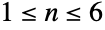
GamblersRuin[p_, n_] := SparseArray[{{1, 1} -> 1, {n + 1, n + 1} -> 1, {i_, j_} /; 1 < i < n + 1 && j == i + 1 -> p, {i_, j_} /; 1 < i < n + 1 && j == i - 1 -> 1 - p}, {n + 1, n + 1}]gamblerwealth = DiscreteMarkovProcess[4, GamblersRuin[0.4, 7]];SeedRandom[2345];ListLinePlot[{#[[1]], #[[2]] - 1}& /@ RandomFunction[gamblerwealth, {0, 30}]["Path"], InterpolationOrder -> 0]Transpose[{MarkovProcessProperties[gamblerwealth, "TransientClasses"][[1]] - 1, MarkovProcessProperties[gamblerwealth, "TransientVisitMean"]}]//TableFormdata = RandomFunction[gamblerwealth, {0, 10 ^ 3}, 10 ^ 4, Method -> {Automatic, "StoppingFunction" -> Function[{len, pos}, len < 1001 && pos ≠ 1 && pos ≠ 8]}]["ValueList"];Table[Mean[Count[#, i]& /@ data], {i, 2, 7}]//NMean[FirstPassageTimeDistribution[gamblerwealth, {1, 8}]]MarkovProcessProperties[gamblerwealth, "TransientTotalVisitMean"]data = DeleteDuplicates /@ RandomFunction[gamblerwealth, {0, 10 ^ 2}, 4 * 10 ^ 3]["ValueList"];Mean[Length[#] - 1& /@ data]//NPDF[gamblerwealth[Infinity], 8]dierolls = DiscreteMarkovProcess[1, With[{numfaces = 6}, SparseArray[{{i_, i_} -> (i - 1) / numfaces, {i_, j_} /; (j - i - 1 == 0) -> (numfaces - (i - 1)) / numfaces}, {numfaces + 1, numfaces + 1}]]];Mean[FirstPassageTimeDistribution[dierolls, 7]]probs = Refine[Probability[x[n] == 7, xdierolls], n > 0]ListPlot[Table[probs, {n, 1, 6 * 6}]]使用正反面概率相同的硬币,求出现序列“反正正”的马可夫过程:
proc1 = DiscreteMarkovProcess[1, {{1 / 2, 1 / 2, 0, 0}, {0, 1 / 2, 1 / 2, 0}, {0, 1 / 2, 0, 1 / 2}, {0, 0, 0, 1}}];Graph[proc1]使用正反面概率相同的硬币,求出现序列“正正正”的马可夫过程:
proc2 = DiscreteMarkovProcess[1, {{1 / 2, 1 / 2, 0, 0}, {1 / 2, 0, 1 / 2, 0}, {1 / 2, 0, 0, 1 / 2}, {0, 0, 0, 1}}];Graph[proc2]FirstPassageTimeDistribution[proc1, 4]//MeanFirstPassageTimeDistribution[proc2, 4]//Mean两个选手打网球,假设发球员赢一个点数的概率是
. 存在 17 种可能的状态:
states = {"GameA", "GameB", "Deux", "AdvA", "AdvB", "40-15", "15-40", "40-0", "30-15", "15-30", "0-40", "30-0", "15-15", "0-30", "15-0", "0-15", "0-0"};proc = With[{p = 3 / 5, q = 2 / 5}, DiscreteMarkovProcess[17, SparseArray[{{1, 1} -> 1, {2, 2} -> 1, {3, 4} -> p, {3, 5} -> q, {4, 1} -> p, {4, 3} -> q, {5, 2} -> q, {5, 3} -> p, {6, 1} -> p, {6, 4} -> q, {7, 2} -> q, {7, 5} -> p, {8, 1} -> p, {8, 6} -> q, {9, 3} -> q, {9, 6} -> p, {10, 3} -> p, {10, 7} -> q, {11, 2} -> q, {11, 7} -> p, {12, 8} -> p, {12, 9} -> q, {13, 9} -> p, {13, 10} -> q, {14, 10} -> p, {14, 11} -> q, {15, 12} -> p, {15, 13} -> q, {16, 13} -> p, {16, 14} -> q, {17, 15} -> p, {17, 16} -> q}, {17, 17}]]];Graph[proc, VertexSize -> Large, VertexLabels -> Thread[Range[17] -> Map[Placed[Style[#, {Bold}], Center]&, states]], ImageSize -> Large, ImagePadding -> 25]PDF[proc[Infinity], 1]//NMarkovProcessProperties[proc, "ReachabilityProbability"][[1]]//NN[Mean[FirstPassageTimeDistribution[proc, {1, 2}]]]Total[MarkovProcessProperties[proc, "TransientVisitMean"]]//NMarkovProcessProperties[proc, "TransientTotalVisitMean"]//NMarkovProcessProperties[proc, "TransientVisitMean"][[1]]//NMean[Count[#, 3]& /@ RandomFunction[proc, {0, 10 ^ 3}, 10 ^ 4, Method -> {Automatic, "StoppingFunction" -> Function[{len, pos}, len < 1001 && pos ≠ 1 && pos ≠ 2]}]["ValueList"]]//N在掷骰子游戏中,玩家掷一对骰子并将点数相加. 第一次投掷时,如果他掷出 7 或者 11,则他获胜,如果掷出 2、3 或者 12 就输了,而任何其他数字称为一个点数,并且继续投掷. 在后面的投掷中,如果玩家掷出点数则获胜,如果掷出 7 则失败. 状态是:开始、赢、输、p4、p5、p6、p8、p9 或 p10. 他从不返回开始状态,而赢和输都是吸收状态. 下面的分布表示投掷一对骰子:
len = Length[Flatten[Map[Permutations, IntegerPartitions[#, {2}, Range[6]]], 1]]& /@ Range[2, 12];dist = ProbabilityDistribution[(len / Total[len]).Map[Boole[k == #]&, Range[2, 12]], {k, 1, 12, 1}];probwin = Probability[x == 7 || x == 11, xdist]problose = Probability[x == 2 || x == 3 || x == 12, xdist]在第一次投掷时他进入“点”状态,如果投出任何其他数字就继续比赛:
probpoint = Probability[x == #, xdist]& /@ {4, 5, 6, 8, 9, 10}problose2 = Probability[x == 7, xdist]probstay = 1 - probpoint - problose2(m = Join[{Join[{0, probwin, problose}, probpoint], UnitVector[9, 2], UnitVector[9, 3]}, Transpose[Join[{ConstantArray[0, Length[probpoint]], probpoint, ConstantArray[problose2, Length[probpoint]]}, DiagonalMatrix[1 - probpoint - problose2]]]])//N//MatrixFormPDF[DiscreteMarkovProcess[1, m][Infinity], {2, 3}]N[%]Mean[FirstPassageTimeDistribution[DiscreteMarkovProcess[1, m], {2, 3}]]N[%]气候 (3)
一个简单的天气模型:给定今天下雨,明天也下雨的概率是 0.7;给定今天没有下雨,明天下雨的概率是 0.4. 给定今天下雨,使用离散马可夫过程表示该模型,求从今天开始下四天雨的概率. 天气的表示:
weather = DiscreteMarkovProcess[1, {{0.7, 0.3}, {0.4, 0.6}}];Graph[weather, VertexLabels -> {1 -> "rain", 2 -> "no rain"}, VertexSize -> Small, EdgeLabels -> With[{sm = MarkovProcessProperties[weather, "TransitionMatrix"]}, Flatten@Table[DirectedEdge[i, j] -> sm[[i, j]], {i, 2}, {j, 2}]], ImageSize -> Medium]Probability[rain[4] == 1, rainweather]基于前两天是否下雨建立一个气候模型. 假设如果今天和昨天下雨,那么明天下雨的概率是 0.7,如果今天下雨但是昨天没有则概率为 0.5,如果昨天下雨今天没有,概率为 0.4,如果昨天或者今天都没下雨,概率是0.2. 使用产品状态空间
,其中
表明昨天是否下雨,
表明今天是否下雨:
rain[{"R", "R"}, {"R", "R"}] = 0.7;
rain[{"R", "R"}, {"R", "N"}] = 1 - 0.7;
rain[{"N", "R"}, {"R", "R"}] = 0.5;
rain[{"N", "R"}, {"R", "N"}] = 1 - 0.5;
rain[{"R", "N"}, {"N", "R"}] = 0.4;
rain[{"R", "N"}, {"N", "N"}] = 1 - 0.4;
rain[{"N", "N"}, {"N", "R"}] = 0.2;
rain[{"N", "N"}, {"N", "N"}] = 1 - 0.2;rain[s_, ns_] := 0m = ArrayFlatten@Table[rain[{x, y}, {z, w}], {x, {"R", "N"}}, {y, {"R", "N"}}, {z, {"R", "N"}}, {w, {"R", "N"}}]TableForm[m, TableHeadings -> {StringJoin /@ Tuples[{"R", "N"}, 2], StringJoin /@ Tuples[{"R", "N"}, 2]}]weather = DiscreteMarkovProcess[1, m];Evaluate[Map[state, StringJoin /@ Tuples[{"R", "N"}, 2]]] = Range[4];Probability[rain[4] == state["RR"] || rain[4] == state["NR"], rainweather]longtermWeather = StationaryDistribution[weather]Probability[rain == state["RR"], rainlongtermWeather]Count[RandomFunction[weather, {1, 10 ^ 4}]["Values"], 1] / 10 ^ 4//N的士要么在机场里,要么在城市中行驶. 从城市出发,下一站是机场的概率是 1/4,或者去城市另一个地方的概率是 3/4. 从机场出发,下一站总是到城市. 使用离散马可夫过程建模,状态1表示城市,状态2表示机场,从机场出发:
taxi = DiscreteMarkovProcess[2, {{3 / 4, 1 / 4}, {1, 0}}];RandomFunction[taxi, {0, 20}]ListPlot[%, Ticks -> {Automatic, {{1, "City"}, {2, "Airport"}}}, Filling -> Axis]dist = StationaryDistribution[taxi]DiscretePlot[PDF[dist, x], {x, {1, 2}}, ExtentSize -> Full, PlotRange -> {{0.5, 2.5}, {0, 1}}, Ticks -> {{1, 2}, Automatic}]容器 (1)
在容器 A 和 B 之间分配
个球,在每一步随机选择一个球,并且转移到另一个容器. 求容器 A 中球的平稳分布. 容器 A 中球的数目使用离散马可夫过程建模. 如果容器 A 中有
个球,A 在失去一个球的概率是
,得到一个球的概率是
,下面是转移矩阵:
(m = With[{n = 10}, Table[Which[j == i - 1, i / n, j == i + 1, 1 - i / n, True, 0], {i, 0, n}, {j, 0, n}]])StationaryDistribution[DiscreteMarkovProcess[1, m]]DiscretePlot[PDF[%, k], {k, 1, 11}, ExtentSize -> 1 / 2]SameQ@@Table[StationaryDistribution[DiscreteMarkovProcess[k, m]], {k, 1, 11}]随机游走 (2)
对于在两端吸收的非延迟随机游走,如果移到右边的几率是 2:1,即使过程从左边界相邻的位置开始,仍然有很好的机会在右边界结束:
PDF[DiscreteMarkovProcess[2, With[{n = 10}, SparseArray[{{1, 1} -> 1, {n, n} -> 1, Band[{2, 1}, {n - 1, n - 2}] -> 1 / 3, Band[{2, 3}] -> 2 / 3}, {n, n}]]][Infinity], {1, 10}]proc = DiscreteMarkovProcess[1, RotateRight[{1 / 3, 1 / 3, 0, 0, 0, 1 / 3},
#] & /@ Range[0, 5]];Graph[proc]MarkovProcessProperties[proc, "Reversible"]MarkovProcessProperties[proc, "Aperiodic"]StationaryDistribution[proc]机器维修 (1)
在一个机器加工车间的一个工作单元中,有三台机器,其中在某一天,一台机器出现故障的概率为 0.1. 机器 1 为机器 2 和 3 提供馈送,如果机器 1 出故障,那么当天无法生产. 一天只能修理一台机器,这样第二天可以使用该机器. 如果几台机器同时出故障,那么它们按优先顺序 1、2和3修理. 假定已经被维修的机器第二天能够运作. 求有一定生产的时间比例. 故障和修理过程可以使用离散马可夫过程建模,通过列出所有可能的故障和正常机器的组合:
failed = Subsets[{1, 2, 3}]transition[i_, j_] /; Length[i] == 0 := p^Length[j](1 - p)^3 - Length[j]一台机器出故障;它被维修,并且剩下的两台机器中一台或者两台可能出故障:
transition[i_, j_] /; Length[i] == 1 := p ^ Length[j](1 - p) ^ (3 - Length[j] - 1)Boole[Unequal@@Join[j, i]]transition[i_, j_] /; Length[i] == 2 && Length[j] == 1 := (1 - p)Boole[Rest[i] == j]transition[i_, j_] /; Length[i] == 2 && Length[j] == 2 := p Boole[And@@Thread[First[i] ≠ j]]transition[i_, j_] /; Length[i] == 2 := 0transition[i_, j_] /; Length[i] == 3 := Boole[j == {2, 3}](m = Block[{p = 0.1}, Table[transition[i, j], {i, failed}, {j, failed}]])//MatrixForm𝒫 = DiscreteMarkovProcess[1, m];Graph[𝒫, GraphLayout -> "BalloonEmbedding"]如果没有机器出故障或者只有机器 2 或 3 出故障,则有产出:
Position[failed, {} | {2} | {3}]Probability[x == 1 || x == 3 || x == 4, xStationaryDistribution[𝒫]]Probability[x == 1, xStationaryDistribution[𝒫]]FirstPassageTimeDistribution[DiscreteMarkovProcess[8, m], 1]//Mean保险 (1)
在最优奖惩汽车保险系统的四状态马可夫链模型中,每个保单持有人有四种状态,取决于前一年索赔的数量,并且这个状态决定了当年的保费. 如果没有索赔通常保费较低,而一个或者多个索赔通常保费较高. 在四个状态的保费金额
下,以及给定保单持有人连续状态的转移矩阵下,如果保单持有人年度索赔量是均值为
的泊松随机变量,求平均年度保费:
policyholderstates = DiscreteMarkovProcess[1, {{a[0], a[1], a[2], 1 - a[0] - a[1] - a[2]}, {a[0], 0, a[1], 1 - a[0] - a[1]}, {0, a[0], 0, 1 - a[0]}, {0, 0, a[0], 1 - a[0]}} /. a[k_] -> PDF[PoissonDistribution[1 / 2], k]]{200, 250, 400, 600}.PDF[StationaryDistribution[policyholderstates], Range[4]]//N其他 (3)
假定一年有 365 天,每天作为生日的概率相等,求使得至少两个人共享一个生日的概率为 50% 的最小人数. 状态有:
— 生日不同的人数
和
— 至少有两人生日相同:
proc = With[{n = 365}, DiscreteMarkovProcess[1, SparseArray[{{n, n + 1} -> 1, {n + 1, n + 1} -> 1, {i_, j_} /; j == i + 1 -> 1 - (i - 1) / n, {i_, n + 1} -> (i - 1) / n}, {n + 1, n + 1}]]];Position[With[{n = 365}, Table[PDF[proc[k], n + 1], {k, 1, 23}]], _ ? (# > 1 / 2&)]//Min考虑一个简单的自然选择模型,其中孤岛的某一物种的总数在食物链上固定为
. 一个变异体存活的概率大于普通个体,在每一代变异体获取一席之地的概率是
,丢失的概率是
:
proc = DiscreteMarkovProcess[2, With[{n = 100}, SparseArray[{{1, 1} -> 1, {n, n} -> 1, Band[{2, 1}, {n - 1, n - 2}] -> 45 / 100, Band[{2, 3}] -> 55 / 100}, {n, n}]]];Probability[nmutants == 100, nmutantsproc[Infinity]]//NMean[FirstPassageTimeDistribution[proc, 100]]//N假设来自火星的无线电信息都以一种这样的语言(只有元音 A 和四个辅音 BCDR)书写,并在普通通信中使用一些通过具有下列估计转移矩阵的马尔可夫链产生的长消息:
sm = {{0, 1 / 2, 1 / 2, 0, 0}, {0, 1 / 3, 0, 1 / 3, 1 / 3}, {0, 0, 1 / 3, 1 / 3, 1 / 3}, {1 / 2, 0, 0, 0, 1 / 2}, {1 / 2, 0, 0, 0, 1 / 2}};proc = DiscreteMarkovProcess[1, sm];1 / PDF[StationaryDistribution[proc], 1]1 / (1 - PDF[StationaryDistribution[proc], 1]){Mean[#], Variance[#]}&[Length /@ DeleteCases[Split[RandomFunction[proc, {0, 10 ^ 5}]["Values"]], {1..} | {3..} | {4..} | {5..}]]N[%]{Mean[#], Variance[#]}&[TransformedDistribution[x + 1, xGeometricDistribution[1 - sm[[2, 2]]]]]N[%]属性和关系 (1)
可能存在的问题 (3)
DiscreteMarkovProcess[1, {{1, 2}, {4, 3}}]DiscreteMarkovProcess[{1, 2}, {{1 / 2, 1 / 2}, {2 / 3, 1 / 3}}]proc = DiscreteMarkovProcess[1, {{(1/2), (1/2), 0, 0, 0}, {(1/3), (2/3), 0, 0, 0}, {0, (1/3), (2/3), 0, 0}, {0, 0, 0, 0, 1}, {0, 0, 0, 1, 0}}];proc[Infinity]MarkovProcessProperties[proc, "Irreducible"]StationaryDistribution[DiscreteMarkovProcess[1, {{(1/2), (1/2), 0, 0, 0}, {(1/3), (2/3), 0, 0, 0}, {0, (1/3), (2/3), 0, 0}, {0, 0, 0, 0, 1}, {0, 0, 0, 1, 0}}]]StationaryDistribution[DiscreteMarkovProcess[4, {{(1/2), (1/2), 0, 0, 0}, {(1/3), (2/3), 0, 0, 0}, {0, (1/3), (2/3), 0, 0}, {0, 0, 0, 0, 1}, {0, 0, 0, 1, 0}}]]文本
Wolfram Research (2012),DiscreteMarkovProcess,Wolfram 语言函数,https://reference.wolfram.com/language/ref/DiscreteMarkovProcess.html (更新于 2014 年).
CMS
Wolfram 语言. 2012. "DiscreteMarkovProcess." Wolfram 语言与系统参考资料中心. Wolfram Research. 最新版本 2014. https://reference.wolfram.com/language/ref/DiscreteMarkovProcess.html.
APA
Wolfram 语言. (2012). DiscreteMarkovProcess. Wolfram 语言与系统参考资料中心. 追溯自 https://reference.wolfram.com/language/ref/DiscreteMarkovProcess.html 年
BibTeX
@misc{reference.wolfram_2026_discretemarkovprocess, author="Wolfram Research", title="{DiscreteMarkovProcess}", year="2014", howpublished="\url{https://reference.wolfram.com/language/ref/DiscreteMarkovProcess.html}", note=[Accessed: 12-September-2026]}
BibLaTeX
@online{reference.wolfram_2026_discretemarkovprocess, organization={Wolfram Research}, title={DiscreteMarkovProcess}, year={2014}, url={https://reference.wolfram.com/language/ref/DiscreteMarkovProcess.html}, note=[Accessed: 12-September-2026]}