FeedbackLinearize[asys]
input-output linearizes the AffineStateSpaceModel asys by state transformation and feedback.
FeedbackLinearize[asys,{z,v}]
specifies the new states z and the new control inputs v.
FeedbackLinearize[asys,{z,v},"prop"]
computes the property "prop".


FeedbackLinearize
FeedbackLinearize[asys]
input-output linearizes the AffineStateSpaceModel asys by state transformation and feedback.
FeedbackLinearize[asys,{z,v}]
specifies the new states z and the new control inputs v.
FeedbackLinearize[asys,{z,v},"prop"]
computes the property "prop".
Details and Options
- FeedbackLinearize is also known as exact linearization.
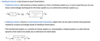
- FeedbackLinearize will construct a linear system lsys from a nonlinear system asys in such a way that you can use linear control design techniques for the linear system lsys to control the nonlinear system asys.
- FeedbackLinearize returns a LinearizingTransformationData object that can be used to extract the properties needed for analysis and design based on feedback linearization.
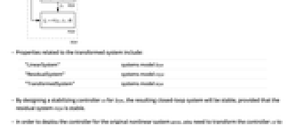
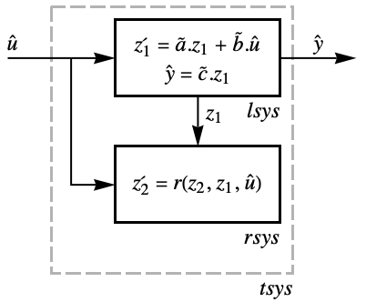
- The transformed system tsys consists of a linear system lsys and possibly a residual system rsys with internal dynamics that need to be stable, but is otherwise not observable.
- Properties related to the transformed system include:
-
"LinearSystem" systems model lsys "ResidualSystem" systems model rsys "TransformedSystem" systems model tsys - By designing a stabilizing controller cs for lsys, the resulting closed-loop system will be stable, provided that the residual system rsys is stable.
- In order to deploy the controller for the original nonlinear system asys, you need to transform the controller cs to use the original variables.
- Properties related to transforming the controller and estimator to original coordinates:
-
{"OriginalSystemController",cs} controller cs in original coordinates {"OriginalSystemEstimator",es} estimator for  and
and 
{"ClosedLoopSystem",cs} closed-loop system in original coordinates {"OriginalSystemFullController",cs} systems model of cs in original coordinates - Further detailed properties of feedback linearization are also available and can be used to deploy alternative simulations and implementations of controllers, estimators, etc.
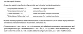
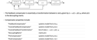
- The system asys
 is connected with a feedback compensator, precompensator, and postcompensator to give a modified system
  , where
  is the modified input,
  is the state vector that consists of
  with possible additional compensator states, and
  is the modified output.
 - The feedback compensator is essentially a transformation between
 and
and  given by
  , where
  is the decoupling matrix.
 - Compensator properties include:
-
"FeedbackCompensator" systems model from  to
to 
"InverseFeedbackCompensator" systems model from  to
to 
"InverseFeedbackTransformation" list of rules 
"DecouplingMatrix" matrix 
"PreCompensator" systems model from  to
to 
"PostCompensator" systems model from  to
to 
- To get an explicitly linear system lsys and a possible residual system rsys, you need to perform a state transformation
 .
. - Properties related to state transformation and zero dynamics include:
-
"InverseStateTransformation" list of rules 
"ZeroDynamicsSystem" systems model 
"ZeroDynamicsManifold" manifold on which the rsys state evolves - FeedbackLinearize takes a Method option with the following settings:
-
Automatic automatically determine method (default) "Identity" apply identity feedback with identity transformation "Burnovsky" return lsys in Burnovsky form


Examples
open all close allBasic Examples (1)
Scope (21)
Basic Uses (5)
Transformed System Properties (1)
Controller and Estimator Properties (5)
Find the nonlinear state feedback controller ![]() :
:
The controller designed using the exactly linearized system:
Obtain the controller ![]() for the original system:
for the original system:
Find a nonlinear state estimator:
Compute the estimator gains for the exactly linearized system:
Obtain the estimator for the original system:
Plot the estimated state trajectories:
Compare the actual and estimated state trajectories:
Find the controlled closed-loop system:
The feedback gains computed using the linearized system:
Obtain the closed-loop system:
Simulate the closed-loop system:
The closed-loop system using a dynamic controller:
The linear controller and estimator design:
The controller for the original system:
The full controller for the original system:
The feedback gains computed using the linearized system:
The full controller for the original system:
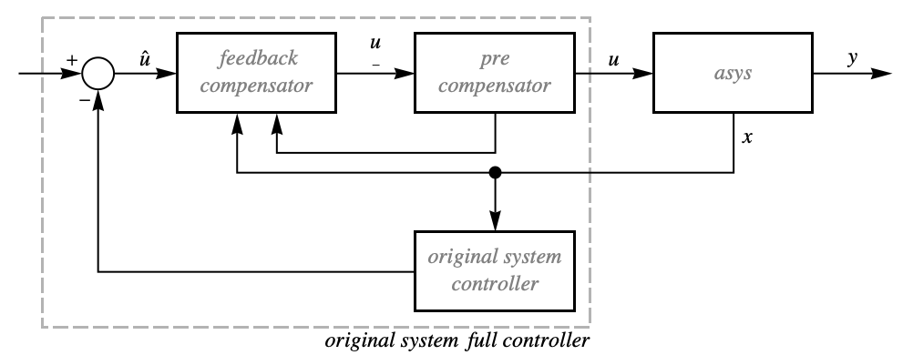
The inputs to the full controller are the reference inputs and the state feedback:
Compensator Properties (5)
The compensated system consists of independent single-input, single-output loops:
The first output is influenced only by the first input:
And the second output is influenced only by the second input:
Other variants of the feedback compensator:
The systems model of the inverse feedback compensator:
The inverse feedback compensator as a list of transformation rules:
The matrix must be invertible for any control design to be valid:
Obtain the decoupling matrix from the inverse feedback transformation:
If possible, a precompensator is computed to make the decoupling matrix nonsingular:
The precompensator in series with the system results in a well-defined vector of relative orders:
The decoupling matrix of just the original system is singular:
If possible, for scalar systems a postcompensator is computed:
With the postcompensator, the system is exactly feedback linearizable:
The post compensator is a combination of the outputs of the system:
Zero Dynamics (5)
It can also be obtained from the residual system by deleting all its inputs:
Compute it from the inverse state transformation:
A system with no residual dynamics rsys:
Since there are no residual dynamics, linear control design can be used:
Simulate a step response for the closed-loop system:
A system with stable residual dynamics:
The residual dynamics are stable, so feedback-design-based linear methods are valid:
Use linear feedback design, and find the feedback law:
A system with unstable residual dynamics rsys:
The eigenvalues have a positive real part, so the rsys is unstable:
For such nonminimum phase systems, the designs based on linear techniques are not valid:
The designed feedback is unable to stabilize the intrinsically ill-behaved system:
Options (2)
Applications (7)
Electromechanical Systems (2)
Design a controller that stabilizes a magnetic levitation system using exact linearization, and compare with a design based on approximate linearization:
The affine model can be obtained directly from the governing equations:
The system without feedback is unstable, here with initial value {0.2,0.,0.1}:
It is completely feedback linearizable, since it has no residual dynamics:
The controller design based on the linear system:
The closed-loop system using original state variables:
Simulate the system with initial value {0.3,0.,0.31305}:
Design based on the approximately linearized system:
The closed-loop system with the controller based on linearization:
Simulation of the system with controller based on approximate linearization:
The design based on feedback linearization has a better response:
Find a stabilizing controller for a two-wheeled inverted pendulum (e.g. Segway) using voltages to the two DC wheel motors as inputs:
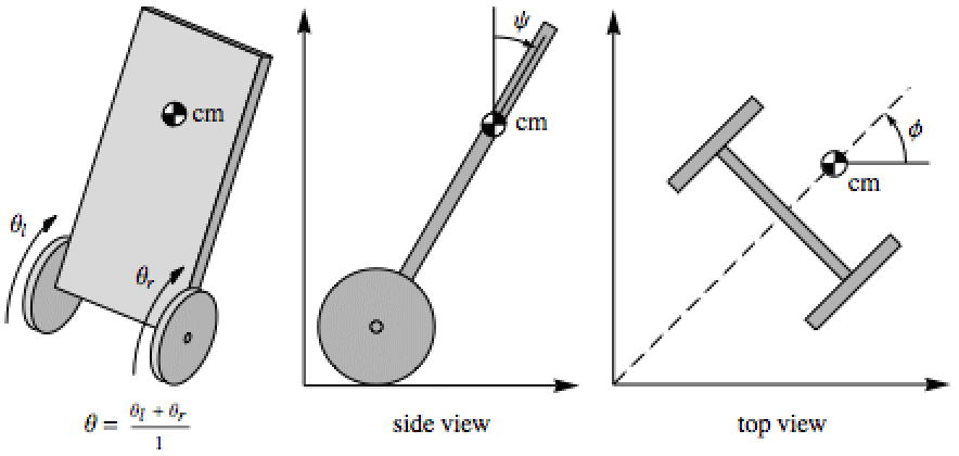
The AffineStateSpaceModel of the system with states {θ,θ',ψ,ψ',ϕ,ϕ'}:
Feedback linearize the system:
The zero dynamics have purely oscillatory behavior:
Design a controller using the linearized subsystem:
Compute the state response of the closed-loop system:
The plots show that the oscillations are in the pendulum's pitch:
Mechanical Systems (2)
Design a vibration controller for a flexible structure, and compute the control effort expended. A two-mode model of a flexible structure with no damping: »
The model is completely feedback linearizable:
Design a controller using the linear system to suppress the vibrations:
The modes of the closed-loop system:
Design a controller to suppress the oscillations in an axial flow compressor. A model of the compressor with throttle as input: »
Simulations show the presence of surge-like oscillations:
Feedback linearize the system:
Design a controller to suppress the oscillations:
Simulations show that the oscillations have been suppressed:
Chemical Systems (1)
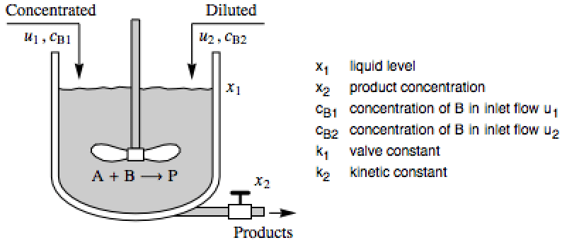
Design a controller to improve an isothermal continuous stirred-tank reactor process: »
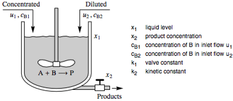
The affine system with states ![]() and inputs
and inputs ![]() :
:
The system is completely feedback linearizable:
Design a controller based on the linearized system:
The response of the closed-loop system from a non-equilibrium initial condition:
The response of the uncontrolled system is far worse:
Assume that the inputs to the system are random and normally distributed:
The response of the controlled system:
Electrical Systems (2)
Design a controller for better speed response in an induction motor subject to varying loads: »

The model of the motor with inputs ![]() :
:
Simulations show the effect of torque on the angular velocity:
The model with an integrator in the q axis:
Feedback linearize the system:
Design a state feedback controller for the linear system:
Simulate the closed-loop system for various torque values:
Design a controller that regulates quantities in a wind energy conversion system: »
The linear system consists of a double integrator and three single integrators:
A controller that gives desired closed-loop transfer functions in each linearized and decoupled loop:
The closed-loop system also has the same linear characteristics plus the zero dynamics:
The response of the system to a unit step applied to each input in turn:
The first input affects only the first output:
And the closed-loop behaves as the designed linear system:
This is true of the three other decoupled SISO loops as well:
Properties & Relations (9)
The linear system lsys is given in Burnovsky form:
The Burnovsky form consists of chains of integrators:
The length of integrator chains is determined by the relative orders:
The Burnovsky form is controllable and observable:
The order of the linear system is the sum of the relative orders:
Since the order of the linear system lsys is less than 4, there are residual dynamics:
The modes of the zero dynamics of a linear system are its transmission zeros:
The problem of zeroing the output:
The trajectories of the zero dynamics:
The inverse state transformation:
Compute the input that gives zero output:
The output is essentially zero for the nonzero input:
The linear system lsys together with the residual system rsys gives the transformed system:
The transformed system tsys has lsys and rsys in parallel:
Obtain it directly from the linearization data object:
Obtain the transformed system from the original system using feedback and coordinate transformation:
It can also be obtained by first applying the transformation and then feedback:
The original system can be reacquired from the transformed system:
The feedback transformation ![]() as a static system:
as a static system:
Apply the feedback followed by the state transform to tsys:
Apply the state transform followed by the feedback to tsys:
The zero dynamics are obtained from the residual dynamics by deleting all the inputs:
Related Guides
History
Text
Wolfram Research (2014), FeedbackLinearize, Wolfram Language function, https://reference.wolfram.com/language/ref/FeedbackLinearize.html.
CMS
Wolfram Language. 2014. "FeedbackLinearize." Wolfram Language & System Documentation Center. Wolfram Research. https://reference.wolfram.com/language/ref/FeedbackLinearize.html.
APA
Wolfram Language. (2014). FeedbackLinearize. Wolfram Language & System Documentation Center. Retrieved from https://reference.wolfram.com/language/ref/FeedbackLinearize.html
BibTeX
@misc{reference.wolfram_2025_feedbacklinearize, author="Wolfram Research", title="{FeedbackLinearize}", year="2014", howpublished="\url{https://reference.wolfram.com/language/ref/FeedbackLinearize.html}", note=[Accessed: 07-May-2026]}
BibLaTeX
@online{reference.wolfram_2025_feedbacklinearize, organization={Wolfram Research}, title={FeedbackLinearize}, year={2014}, url={https://reference.wolfram.com/language/ref/FeedbackLinearize.html}, note=[Accessed: 07-May-2026]}