

LQOutputRegulatorGains
LQOutputRegulatorGains[sspec,wts]
重み wts で出力費用関数を最小にする系の指定 sspec のための状態フィードバックゲインを与える.
LQOutputRegulatorGains[…,"prop"]
特性"prop"の値を与える.
詳細とオプション
- LQOutputRegulatorGainsは,線形二次出力調整器,線形二次出力コントローラ,あるいは最適コントローラとしても知られている.
- LQOutputRegulatorGainsは,系を安定させたりその性能を向上させたりするためによく使われる.
- 通常,コントローラは状態フィードバック
 で与えられる.ただし,
 は計算されたフィードバックゲイン行列である.
- sys の入力 u はフィードバック入力 ufと,場合によってはその他の入力 ueからなる.
- sys の出力 y は調整された出力 yrと,場合によってはその他の出力からなる.
- 系の指定 sspec は指定 ufと yrを含む系 sys である.
- LQOutputRegulatorGainsは,調整された出力 yrの重み q, r, p と線形系 sys のフィードバック入力 ufを使って二次費用関数を最小化する.
-

連続時間系 
離散時間系 - LQ設計はStateSpaceModelで指定されているように線形系に使うことができる.
-

連続時間系 
離散時間系 - 結果のフィードバックゲイン行列は
 として計算される.
-


連続時間系 

離散時間系 - 行列 xrはリッカティ(Riccati)方程式の解である.
-

連続時間代数リッカティ方程式 
離散時間代数リッカティ方程式 - 部分行列 bf, cr, drfはフォードバック入力 ufと調整された出力 yrに対応する.
- 重み wts は次の形でよい.
-
{q,r} クロスカップリングがない費用関数 {q,r,p} クロスカップリング行列 p がある費用関数 - 系の指定 sspec は以下の形でよい.
-
StateSpaceModel[…] 線形制御入力と線形状態 AffineStateSpaceModel[…] 線形制御入力と非線形状態 NonlinearStateSpaceModel[…] 非線形制御入力と非線形状態 SystemModel[…] 一般的な系のモデル <…> Associationとして与えられる詳細な系の指定 - 系の指定の詳細は次のキーを持つことができる.
-
"InputModel" sys モデルの任意のもの "FeedbackInputs" All フィードバック入力 uf "RegulatedOutputs" All 調整された出力 yr - 入力と出力は以下の形でよい.
-
{num1,…,numn} StateSpaceModel,AffineStateSpaceModel,NonlinearStateSpaceModelで使われる番号付きの入力または出力 numi {name1,…,namen} SystemModelで使われる名前付きの入力または出力 namei All すべての入力または出力を使う - AffineStateSpaceModel,NonlinearStateSpaceModel,SystemModelのような非線形系については, 系は保存された動作点の周りで線形化される.
- LQOutputRegulatorGains[…,"Data"]は,cd["prop"]の形で追加的な特性の抽出に使えるSystemsModelControllerDataオブジェクト cd を返す.
- LQOutputRegulatorGains[…,"prop"]を使って cd["prop"]の値を直接得ることができる.
- 次は,特性"prop"の可能な値である.
-
"ClosedLoopPoles" 線形化された"ClosedLoopSystem"の極 "ClosedLoopSystem" ueと  を入力として,y を出力として持つ系 csys
{"ClosedLoopSystem", cspec} 閉ループ系の形に対する詳細な制御 "ControllerModel"  と x を入力として,ufを出力として持つモデル cm
"Design" コントローラ設計のタイプ "DesignModel" 設計に使われるモデル "FeedbackGains" ゲイン行列 κ またはそれに相当するもの "FeedbackGainsModel" x を入力として,  を出力として持つモデル gm
"FeedbackInputs" フィードバックに使われる sys の入力 uf "InputModel" 入力モデル sys "InputCount" sys の入力 u の数 "OpenLoopPoles" "DesignModel"の極 "OutputCount" sys の出力 y の数 "RegulatedOutputs" sys の調整された出力 yr "SamplingPeriod" sys のサンプリング周期 "StateCount" sys の状態 x の数 - 次は,cspec の可能なキーである.
-
"InputModel" csys の入力モデル "Merge" csys をマージするかどうか "ModelName" csys の名前
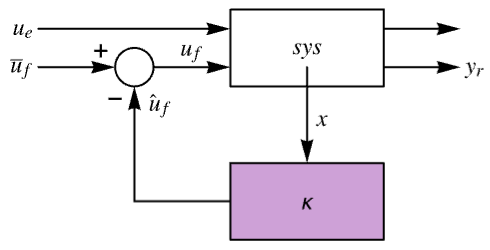
以下は,フィードバックゲインモデル gm,コントローラモデル cm,閉ループ系 csys の線図である.
[image]例題
すべて開く すべて閉じる例 (2)
連続時間系についての出力に重みの付いた最適状態フィードバックゲインの集合:
LQOutputRegulatorGains[StateSpaceModel[{{{0, 1, 0}, {0, -0.01, 0.3}, {0, -0.003, -10}}, {{0, 0}, {0, -1}, {0.1, 0}},
  {{1, 0, 0}, {0, 1, 0}}, {{1, 0}, {0, 1}}}, SamplingPeriod -> None, SystemsModelLabels -> None], {(|   |   |
| - | - |
| 1 | 0 |
| 0 | 1 |), (|     |     |
| --- | --- |
| 0.1 | 0   |
| 0 | 0.1 |)}]//MatrixFormLQOutputRegulatorGains[StateSpaceModel[{{{-0.05156, -0.05877}, {0.01503, -0.005887}}, {{0}, {-0.03384}},
{{1.1, -0.5}, {-0.7, 1}}, {{0.1}, {0.2}}}, SamplingPeriod -> 0.1, SystemsModelLabels -> None], {(| | |
| -- | --- |
| 10 | 0 |
| 0 | 0.1 |), {{1}}}]スコープ (27)
基本的な用法 (8)
入出力の等しい重みを使って系の状態フィードバックゲインを計算する:
ssm = StateSpaceModel[{{{-10}}, {{1}}, {{1}}, {{1}}}, SamplingPeriod -> None, SystemsModelLabels -> None];κ = LQOutputRegulatorGains[ssm, {{{1}}, {{1}}}]SystemsModelStateFeedbackConnect[ssm, κ]//Simplifyssm = StateSpaceModel[{{{10}}, {{1}}, {{1}}, {{1}}}, SamplingPeriod -> None, SystemsModelLabels -> None];κ = LQOutputRegulatorGains[ssm, {{{1}}, {{1}}}]SystemsModelStateFeedbackConnect[ssm, κ]//Simplifyssm = StateSpaceModel[{{{0, 0, -0.1}, {1., 0., -1.08}, {0., 1., -0.9}}, {{1}, {1}, {0}},
{{0, 1, 1}, {0, 0, 1}}, {{0}, {0}}}, SamplingPeriod -> None, SystemsModelLabels -> None];κ = LQOutputRegulatorGains[ssm, {(| | |
| - | - |
| 1 | 0 |
| 0 | 2 |), (0.5)}]Dimensions[κ]{SystemsModelDimensions[ssm][[1]], SystemsModelOrder[ssm]}ssm = StateSpaceModel[{{{0, 0, -0.1, 0}, {1., 0., -1.08, 0.1}, {0., 1., -0.9, -1}, {0, 1, 0, 0}},
{{1, 0}, {0, 1}, {0, 0}, {0, 0}}, {{1, 0, 0, 1}, {0, 1, 0, 1}, {0, 0, 1, 1}},
{{0, 0}, {0, 0}, {0, 0}}}, SamplingPeriod -> None, SystemsModelLabels -> None];MatrixForm[κ1 = LQOutputRegulatorGains[ssm, {(| | | |
| - | - | -- |
| 1 | 0 | 0 |
| 0 | 1 | 0 |
| 0 | 0 | 10 |), (| | |
| - | - |
| 1 | 0 |
| 0 | 5 |)}]]MatrixForm[κ2 = LQOutputRegulatorGains[ssm, {(| | | |
| - | - | -- |
| 1 | 0 | 0 |
| 0 | 1 | 0 |
| 0 | 0 | 10 |), (| | |
| - | - |
| 5 | 0 |
| 0 | 1 |)}]]一般に,より重みが大きいフィードバック入力の方がノルムが小さい:
Norm /@ κ1
Norm /@ κ2
費用関数が出力とフィードバック入力のクロスカップリングを含む場合のゲインを計算する:
ssm = StateSpaceModel[{{{0, 0, -0.1}, {1., 0., -1.08}, {0., 1., -0.9}}, {{1, 1}, {1, 0}, {0, 0}},
{{1, 0, 1}}, {{0, 0}}}, SamplingPeriod -> None, SystemsModelLabels -> None];LQOutputRegulatorGains[ssm, {(1), (| | |
| - | - |
| 1 | 0 |
| 0 | 1 |), (0.1 0.1)}]//MatrixFormssm = StateSpaceModel[{{{0, 1., 0.}, {0, 0., 1.}, {-0.1, -1.08, -0.9}}, {{0}, {0}, {1}},
{{1, 1, 0}, {1, 0, 0}}, {{0}, {0}}}, SamplingPeriod -> None, SystemsModelLabels -> None];wts = {(1), (5)};LQOutputRegulatorGains[<|"InputModel" -> ssm, "RegulatedOutputs" -> 1|>, wts]LQOutputRegulatorGains[<|"InputModel" -> ssm, "RegulatedOutputs" -> 2|>, wts]ssm = StateSpaceModel[{{{0, 0, -0.1}, {1., 0., -1.08}, {0., 1., -0.9}}, {{1, 1}, {1, 0}, {0, 0}},
{{1, 0, 1}}, {{0, 0}}}, SamplingPeriod -> None, SystemsModelLabels -> None];wts = {(1), (5)};LQOutputRegulatorGains[<|"InputModel" -> ssm, "FeedbackInputs" -> 1|>, wts]LQOutputRegulatorGains[<|"InputModel" -> ssm, "FeedbackInputs" -> 2|>, wts]nssm = NonlinearStateSpaceModel[{{u + x + x^2},
{-1 + x}}, {{x, 1}}, {{u, -2}}, {Automatic}, Automatic,
SamplingPeriod -> None];LQOutputRegulatorGains[nssm, {{{10}}, {{1}}}]LQOutputRegulatorGains[StateSpaceModel[nssm], {{{10}}, {{1}}}]工場モデル (6)
連続時間StateSpaceModel:
LQOutputRegulatorGains[StateSpaceModel[{{{0, 1.}, {-1, -1.6}}, {{0}, {1}}, {{1, 1}, {0, 1}}, {{0}, {0}}},
SamplingPeriod -> None, SystemsModelLabels -> None], {(| | |
| - | - |
| 1 | 0 |
| 0 | 1 |), (1)}]離散時間StateSpaceModel:
LQOutputRegulatorGains[StateSpaceModel[{{{0, 1.}, {0.020000000000000004, 0.1}}, {{0}, {1}}, {{1, 1}, {0, 1}}, {{0}, {0}}},
SamplingPeriod -> τ, SystemsModelLabels -> None], {(| | |
| - | - |
| 1 | 0 |
| 0 | 1 |), (1)}]ディスクリプタStateSpaceModel:
LQOutputRegulatorGains[StateSpaceModel[{{{-6, -4}, {-6, -5}}, {{1}, {1}}, {{1, 1}, {0, 1}}, {{0}, {0}}, {{1, 1}, {0, 1}}},
{{x1[t], 0}, {x2[t], 0}},
{{u[t], 0}}, Automatic, t, SamplingPeriod -> None,
SystemsModelLabels -> None], {(| | |
| - | - |
| 1 | 0 |
| 0 | 1 |), (1.0)}]LQOutputRegulatorGains[AffineStateSpaceModel[{{Sin[Subscript[x, 1]] + Subscript[x, 2],
-Subscript[x, 1] - Subscript[x, 2]},
{{Subscript[x, 1]}, {1}},
{Subscript[x, 1] - Subscript[x, 2], Subscript[x, 2]},
{{0}, {0}}}, {Subscript[x, 1], Subscript[x, 2]}, {{u, 0}},
{Automatic, Automatic}, Automatic, SamplingPeriod -> None], {(| | |
| - | - |
| 1 | 0 |
| 0 | 1 |), (1.0)}]LQOutputRegulatorGains[NonlinearStateSpaceModel[
{{Subscript[x, 2] + Subscript[x, 1]*Subscript[x, 2],
u + Subscript[x, 1]},
{Subscript[x, 1] - Subscript[x, 2], Subscript[x, 2]}},
{Subscript[x, 1], Subscript[x, 2]}, {u},
{Automatic, Automatic}, Automatic, SamplingPeriod -> None], {(| | |
| - | - |
| 1 | 0 |
| 0 | 1 |), (1.0)}]sm = CreateSystemModel[{x''[t] + x'[t] + x[t] == u[t], y1[t] == x[t], y2[t] == x'[t]}, t, {"u"∈"Modelica.Blocks.Interfaces.RealInput", {"y1", "y2"}∈"Modelica.Blocks.Interfaces.RealOutput"}];LQOutputRegulatorGains[sm, {(| | |
| - | - |
| 1 | 0 |
| 0 | 1 |), (1)}]特性 (10)
LQOutputRegulatorGainsは,デフォルトでフィードバックゲインを返す:
ssm = StateSpaceModel[{{{0, 1}, {-1, -2}}, {{0}, {1}}, {{1, 1}}, {{0}}}, SamplingPeriod -> None,
SystemsModelLabels -> None];wts = {(1.0), (1.0)};LQOutputRegulatorGains[ssm, wts]% == LQOutputRegulatorGains[ssm, wts, "FeedbackGains"]κ = LQOutputRegulatorGains[NonlinearStateSpaceModel[
{{-Subscript[x, 1] + u*Subscript[x, 1] +
Subscript[x, 2]/E^Subscript[x, 1],
E^Subscript[x, 2] - Subscript[x, 1]},
{u + Subscript[x, 1], Subscript[x, 2]}},
{{Subscript[x, 1], 1}, {Subscript[x, 2], 0}}, {{u, 1.}},
{Automatic, Automatic}, Automatic, SamplingPeriod -> None], {(| | |
| - | - |
| 1 | 0 |
| 0 | 1 |), (1)}]これは κ0+κ1.x の形をしている.κ0と κ1は定数である:
{κ0, κ1} = {κ /. {Subscript[x, _] -> 0}, D[κ, {{Subscript[x, 1], Subscript[x, 2]}}]}LQOutputRegulatorGains[StateSpaceModel[{{{0, 1}, {-1, -2}}, {{0}, {1}}, {{1, 1}}, {{0}}}, SamplingPeriod -> None,
SystemsModelLabels -> None], {(1.0), (1.0)}, "FeedbackGainsModel"]LQOutputRegulatorGains[NonlinearStateSpaceModel[{{Subscript[x, 2], -2/3 + u -
Subscript[x, 1]/3 - Subscript[x, 2]/2},
{Subscript[x, 1] + Subscript[x, 2]}},
{{Subscript[x, 1], 1}, {Subscript[x, 2], 0}}, {{u, 1.}},
{Automatic}, Automatic, SamplingPeriod -> None], {(1.0), (1.0)}, "FeedbackGainsModel"]//ChopLQOutputRegulatorGains[StateSpaceModel[{{{0., 1.}, {-0.05, -0.9}}, {{0}, {1}}, {{1, 1}, {0, 1}}, {{0}, {0}}},
{Subscript[x, 1], Subscript[x, 2]}, {{f, 0}},
SamplingPeriod -> None, SystemsModelLabels -> None], {(| | |
| - | - |
| 1 | 0 |
| 0 | 1 |), (1)}, "ClosedLoopSystem"]assm = AffineStateSpaceModel[{{Subscript[x, 2], -0.05*Subscript[x, 1] -
0.9*Subscript[x, 2]^2}, {{0}, {1}},
{Subscript[x, 1] + Subscript[x, 2], Subscript[x, 2]},
{{0}, {0}}}, {Subscript[x, 1], Subscript[x, 2]}, {{f, 0}},
{Automatic, Automatic}, Automatic, SamplingPeriod -> None];
wts = {(| | |
| - | - |
| 1 | 0 |
| 0 | 1 |), (1)};LQOutputRegulatorGains[assm, wts, "ClosedLoopPoles"]assm = AffineStateSpaceModel[{{Subscript[x, 2], -0.05*Subscript[x, 1] -
0.9*Subscript[x, 2]^2}, {{0}, {1}},
{Subscript[x, 1] + Subscript[x, 2], Subscript[x, 2]},
{{0}, {0}}}, {Subscript[x, 1], Subscript[x, 2]}, {{f, 0}},
{Automatic, Automatic}, Automatic, SamplingPeriod -> None];
wts = {(| | |
| - | - |
| 1 | 0 |
| 0 | 1 |), (1)};dmodel = LQOutputRegulatorGains[assm, wts, "DesignModel"]LQOutputRegulatorGains[dmodel, wts]
LQOutputRegulatorGains[assm, wts]LQOutputRegulatorGains[AffineStateSpaceModel[{{Subscript[x, 2], -0.05*Subscript[x, 1] -
0.9*Subscript[x, 2]^2}, {{0}, {1}},
{Subscript[x, 1] + Subscript[x, 2], Subscript[x, 2]},
{{0}, {0}}}, {Subscript[x, 1], Subscript[x, 2]}, {{f, 0}},
{Automatic, Automatic}, Automatic, SamplingPeriod -> None], {(| | |
| - | - |
| 1 | 0 |
| 0 | 1 |), (1)}, "Design"]Dataset[Table[{prop, LQOutputRegulatorGains[IconizedObject[«sys»], IconizedObject[«wts»], prop]}, {prop, IconizedObject[«props»]}]]𝒸𝒹 = LQOutputRegulatorGains[IconizedObject[«sys»], IconizedObject[«wts»], "Data"]𝒸𝒹["Properties"]𝒸𝒹["ClosedLoopPoles"]閉ループ系 (3)
assm = AffineStateSpaceModel[{{Subscript[x, 1] - Subscript[x, 1]^2 -
    Subscript[x, 2], Subscript[x, 1]}, {{0}, {1}},
  {Subscript[x, 1] + Subscript[x, 2]}, {{0}}},
 {Subscript[x, 1], Subscript[x, 2]}, {u}, {Automatic},
Automatic, SamplingPeriod -> None];csys1 = LQOutputRegulatorGains[assm, {(1.0), (1.0)}, "ClosedLoopSystem"]csys2 = LQRegulatorGains[assm, {(| | |
| - | - |
| 1 | 0 |
| 0 | 1 |), (1.0)}, {"ClosedLoopSystem", <|"InputModel" -> AffineStateSpaceModel[{{Subscript[x, 1] - Subscript[x, 2],
Subscript[x, 1]}, {{0}, {1}},
{Subscript[x, 1] + Subscript[x, 2]}, {{0}}},
{Subscript[x, 1], Subscript[x, 2]}, {u}, {Automatic},
Automatic, SamplingPeriod -> None]|>}]Table[OutputResponse[{sys, {0.5, 1}}, 0, {t, 0, 7}], {sys, {csys1, csys2}}];
Plot[%, {t, 0, 7}, PlotLegends -> {"Nonlinear", "Linear"}, PlotRange -> All]1つの外乱と1つのフィードバック入力を使用して,工場のマージされた閉ループ系を組み立てる:
sys = <|"InputModel" -> StateSpaceModel[{{{0., 1.}, {-0.05, -0.9}}, {{0, 0}, {1, 1}}, {{1, 1}}, {{0, 0}}},
 {Subscript[x, 1], Subscript[x, 2]},
 {{d, 0}, {f, 0}}, SamplingPeriod -> None,
 SystemsModelLabels -> {{Subscript[u, e],
Subscript[u, f]}}], "FeedbackInputs" -> 2|>;wts = {(1.0), (1.0)};LQOutputRegulatorGains[sys, wts, "ClosedLoopSystem"]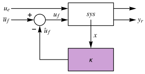
LQOutputRegulatorGains[sys, wts, {"ClosedLoopSystem", <|"Merge" -> False|>}]SystemsModelMerge[%]LQOutputRegulatorGains[sys, wts, {"ClosedLoopSystem", <|"Merge" -> True|>}]sm = CreateSystemModel["MassSpringDamper", {m x''[t] + c x'[t] + k x[t] == u[t], y1[t] == x[t], y2[t] == x'[t]}, t, {"u"∈"Modelica.Blocks.Interfaces.RealInput", {"y1", "y2"}∈"Modelica.Blocks.Interfaces.RealOutput"}, <|"ParameterValues" -> {m -> 10, c -> 10^2, k -> 10^3}|>];csysName = "MassSpringDamperWithStateFeedback";csys = LQOutputRegulatorGains[sm, {(| | |
| - | - |
| 1 | 0 |
| 0 | 1 |), (1)}, {"ClosedLoopSystem", <|"ModelName" -> csysName|>}]csys["ModelName"]この名前を直接使って他の関数の閉ループモデルを指定することができる:
SystemModelSimulate[csysName, {"y1", "y2"}, 2, <|"Inputs" -> {"u" -> UnitStep}|>]SystemModelPlot[%, All, PlotRange -> All]アプリケーション (2)
航空機モデルの出力に重みの付いた状態フィードバックゲイン行列を構築する:
aircraftM = StateSpaceModel[{{{0.4158, 1.025, -0.00267, -0.00011106, -0.08021, 0},
   {-5.5, -0.8302, -0.06549, -0.0039, -5.115, 0.809}, {0, 0, 0, 1, 0, 0},
   {-1040, 78.35, -34.83, -0.6214, -865.6, -631}, {0, 0, 0, 0, -75, 0}, {0, 0, 0, 0, 0, -100}},
  {{0, 0}, {0, 0}, {0, 0}, {0, 0}, {75, 0}, {0, 100}}, {{1, 0, 0, 0, 2, 0}, {0, 1, 0, 0, 0, 0}},
{{0, 0}, {0, 0}}}, SamplingPeriod -> None, SystemsModelLabels -> None];k = LQOutputRegulatorGains[aircraftM, {(| | |
| ------ | - |
| 0.0001 | 0 |
| 0 | 1 |), (| | |
| - | - |
| 1 | 0 |
| 0 | 1 |)}]aircraftMCL = SystemsModelStateFeedbackConnect[aircraftM, k];or = OutputResponse[{aircraftMCL, {0, 0.1, 0, 0, 0, 0}}, {0, 0}, {t, 0, 6}];Plot[or, {t, 0, 6}, PlotRange -> All, PlotLegends -> {Subscript[y, 1], Subscript[y, 2]}]fb = -k.StateResponse[{aircraftMCL, {0, 0.1, 0, 0, 0, 0}}, {0, 0}, {t, 6}];Plot[fb, {t, 0, 6}, PlotRange -> All, PlotLegends -> {Subscript[u, 1], Subscript[u, 2]}]circuit = StateSpaceModel[{{{0, 0, 0, 1}, {0, 0, 1, 0}, {-1, 1, 0, 0}, {1, 0, 10, 10}},
{{0}, {0}, {0}, {-1}}, {{0, 0.1, 0, 0}}, {{0}}, {{0.1, 0, 0, 0}, {0, 0.2, 0, 0},
{0, 0, -0.01, 0}, {0, 0, 0, 0}}}, Automatic, SamplingPeriod -> None, SystemsModelLabels -> None];openloopresponse = OutputResponse[circuit, Sin[6 2 Pi t], {t, 0, 1}];
Plot[openloopresponse, {t, 0, 1}, PlotRange -> All]k = LQOutputRegulatorGains[circuit, {{{1}}, {{1}}}];
clssm = SystemsModelStateFeedbackConnect[circuit, k]closedloopresponse = OutputResponse[clssm, Sin[6 2 Pi t], {t, 0, 1}];
Plot[closedloopresponse, {t, 0, 1}, PlotRange -> All]特性と関係 (3)
LQRegulatorGainsを使って同等な出力調整器ゲインを計算することができる:
{a, b, c, d} = {(| | | |
| -- | -- | -- |
| -2 | 0 | 1 |
| 0 | -1 | 0 |
| -3 | -4 | -2 |), (| | |
| - | - |
| 0 | 1 |
| 0 | 0 |
| 1 | 0 |), (| | | |
| - | - | - |
| 1 | 0 | 0 |
| 0 | 1 | 0 |), (| | |
| - | - |
| 1 | 0 |
| 0 | 2 |)};{q, r, p} = {(| | |
| --- | --- |
| 100 | 0. |
| 0 | 0.1 |), (| | |
| -- | - |
| 10 | 0 |
| 0 | 1 |), (| | |
| - | - |
| 1 | 0 |
| 0 | 1 |)};ssm = StateSpaceModel[{a, b, c, d}];LQRegulatorGains[ssm, {c.q.c, r + d.q.d + d.p + p.d, c.q.d + c.p}]LQOutputRegulatorGainsも同じ結果を与える:
LQOutputRegulatorGains[ssm, {q, r, p}] - %もとになっているリッカティ方程式を解くことで線形二次出力調整器ゲインを計算する:
{a, b, c, d} = {(| | | | | |
| - | -------- | ------- | - | ------- |
| 0 | -0.01156 | -0.1711 | 0 | 0 |
| 0 | -0.1419 | 0.1711 | 0 | 0 |
| 0 | -0.00875 | -1.102 | 0 | 0 |
| 0 | -0.00128 | -0.1489 | 0 | 0.00013 |
| 0 | 0.0605 | 0.1489 | 0 | -0.0591 |), (| | | |
| ----- | ------- | ------- |
| 0 | -0.143 | 0 |
| 0 | 0 | 0 |
| 0.392 | 0 | 0 |
| 0 | 0.108 | -0.0592 |
| 0 | -0.0486 | 0 |), (| | | | | |
| - | - | - | - | - |
| 1 | 0 | 0 | 0 | 0 |
| 0 | 0 | 0 | 1 | 0 |
| 0 | 0 | 0 | 0 | 1 |), (| | | |
| - | - | - |
| 0 | 1 | 0 |
| 1 | 0 | 0 |
| 0 | 0 | 1 |)};{q, r, p} = {(| | | |
| ---- | --- | -- |
| 1000 | 0 | 0 |
| 0 | 100 | 0 |
| 0 | 0 | 10 |), (| | | |
| - | - | -- |
| 1 | 0 | 0 |
| 0 | 1 | 0 |
| 0 | 0 | 10 |), (| | | |
| --- | - | - |
| 100 | 0 | 0 |
| 0 | 1 | 0 |
| 0 | 0 | 1 |)};With[{q = c.q.c, r = r + d.q.d + d.p + p.d, p = c.q.d + c.p}, Inverse[r].(b.RiccatiSolve[{a, b}, {q, r, p}] + p)]LQOutputRegulatorGainsも同じ結果を与える:
LQOutputRegulatorGains[StateSpaceModel[{a, b, c, d}], {q, r, p}] - %//ChopDiscreteRiccatiSolveを使って離散時間系のゲインを計算する:
{a, b, c, d} = {(| | | | | |
| - | -------- | ------- | - | ------- |
| 1 | -0.01866 | -0.134 | 0 | 0 |
| 0 | 0.7516 | 0.1144 | 0 | 0 |
| 0 | -0.0059 | 0.1097 | 0 | 0 |
| 0 | -0.0009 | -0.1203 | 1 | 0.00025 |
| 0 | 0.0978 | 0.1206 | 0 | 0.8885 |), (| | | |
| ------- | ------- | ------- |
| -0.0732 | -0.286 | 0 |
| 0.0652 | 0 | 0 |
| 0.3162 | 0 | 0 |
| -0.0632 | 0.216 | -0.1184 |
| 0.0634 | -0.0917 | 0 |), (| | | | | |
| - | - | - | - | - |
| 1 | 0 | 0 | 0 | 0 |
| 0 | 0 | 0 | 1 | 0 |
| 0 | 0 | 0 | 0 | 1 |), (| | | |
| - | - | - |
| 0 | 1 | 0 |
| 1 | 0 | 0 |
| 0 | 0 | 1 |)};{q, r, p} = {(| | | |
| ---- | --- | -- |
| 1000 | 0 | 0 |
| 0 | 100 | 0 |
| 0 | 0 | 10 |), (| | | |
| - | - | -- |
| 1 | 0 | 0 |
| 0 | 1 | 0 |
| 0 | 0 | 10 |), (| | | |
| --- | - | - |
| 100 | 0 | 0 |
| 0 | 1 | 0 |
| 0 | 0 | 1 |)};With[{q = c.q.c, r = r + d.q.d + d.p + p.d, p = c.q.d + c.p}, With[{x = DiscreteRiccatiSolve[{a, b}, {q, r, p}]}, Inverse[b.x.b + r].(b.x.a + p)]]LQOutputRegulatorGainsも同じ結果を与える:
LQOutputRegulatorGains[StateSpaceModel[{a, b, c, d}, SamplingPeriod -> τ], {q, r, p}] - %//Chopテキスト
Wolfram Research (2010), LQOutputRegulatorGains, Wolfram言語関数, https://reference.wolfram.com/language/ref/LQOutputRegulatorGains.html (2021年に更新).
CMS
Wolfram Language. 2010. "LQOutputRegulatorGains." Wolfram Language & System Documentation Center. Wolfram Research. Last Modified 2021. https://reference.wolfram.com/language/ref/LQOutputRegulatorGains.html.
APA
Wolfram Language. (2010). LQOutputRegulatorGains. Wolfram Language & System Documentation Center. Retrieved from https://reference.wolfram.com/language/ref/LQOutputRegulatorGains.html