Modelica Aspects and Modeling Advice
This chapter explains some important aspects of the Modelica language and gives you advice on things to keep in mind when working with System Modeler.
Model Initialization
At the start time of a model simulation, the model needs to be initialized, which typically involves calculating values for more variables than the integration problem. Specifically, in addition to the variables calculated during integration, states, parameters with fixed=false and pre values for discrete variables need to have values calculated for them.
System Modeler detects three different kinds of initialization:
The equations used during initializations are all initial equations and initial algorithms in the model, in addition to all regular equations and algorithms (when equations and when statements are special cases; see later section). Also, any variables with fixed=true are counted as one equation (see the section on the fixed attribute).
The kind of initialization used is dependent on the initialization settings you have in your model. Determined initialization is the preferred outcome for a model, because System Modeler did not find any conflicts nor did it need to choose which variables should be initialized from their start values.
In underdetermined initialization, System Modeler had too few equations and had to choose some variables to be initialized from their start values. In this case, there is a notification issued that can be seen in the Build Log in SimulationCenter, showing which variables System Modeler chose.
In overdetermined initialization, System Modeler had too many equations or found conflicting equations. In this case, a warning is issued in the Build Log in SimulationCenter. It is recommended to not use overdetermined initialization and fix any models that have it.
Start Attribute
All variables in Modelica have a start value. If you do not specify a start value for a variable, it has a default start value depending on the type: 0.0 for Real, 0 for Integer and false for Boolean.
Start values can be used for two things. They can be used to initialize a variable exactly to that value, or they can be used as a guess value for a variable solved in a nonlinear system. You can see variable start values and how they are used in the Variables tab in SimulationCenter.
If your model has underdetermined initialization, there are too few equations and System Modeler has to pick some variables to be initialized from their start values. System Modeler does this by checking which variables can be initialized from the start, given the equation structure of the model, and then choosing the variables it considers most suitable. System Modeler considers variables that have a specified start value more suitable and considers states to be more suitable than other variables. In the model A, System Modeler will choose to initialize x to its start value.
model A
  Real x(start = 1);
equation
  der(x) = -x + 1;
end A;
When a start value is used as a guess value, it can help you get the solution you want. Consider the equation z2-6=z, which has two solutions, z=2 and z=3. In the models B1 and B2, you can see that different solutions are found, depending on your start setting.
model B1
 Real z(start = 4);
equation
 z^2 = 6 - z;
end B1;
model B2
 Real z(start = -5);
equation
 z^2 = 6 - z;
end B2;
Initial Equations and Algorithms
The easiest way to set a variable's value at start time is to use an initial equation or an initial algorithm.
model C
  Real x;
initial algorithm
  x := 1;
equation
  der(x) = -x + 1;
end C;
In the model C, x will always start with its value equal to 1, while in the model A, the start value of x could easily be changed by a modification or by changing the start value in the Variables tab in SimulationCenter. It is not possible to change an initial equation section by a modification. An initial equation section is in some ways more powerful than the start attribute, since you can use full equations to express initial constraints. For example, in the model D, the variable x will start in steady state, since der(x)=0 is used as an initial equation.
model D
  Real x;
  Real y(start = 3);
initial equation
  der(x) = 0;
equation
  der(x) = -x + y + 1;
  der(y) = -y +2;
end D;
Fixed Attribute
The fixed attribute can be added to a variable declaration to say that the variable should be initialized exactly to its start value. Effectively, this is the same as adding an initial equation. However, if you use fixed=true and the start value is a literal number, you can change it after the simulation has been built in the Variables tab in SimulationCenter. The two models following, HelloWorld and HelloWorldInitialEquation, show the difference.
model HelloWorld
  Real x(fixed = true, start = 1.0);
equation
  der(x) = -x;
end HelloWorld;
model HelloWorldInitialEquation
  Real x;
initial equation
  x = 1.0;
equation
  der(x) = -x;
end HelloWorldInitialEquation;
For parameters, you can set fixed=false to indicate that a parameter should be calculated during initialization. In the model HelloWorldParameter, the exponential decay constant is a parameter that is calculated at initialization; specifically, it will be two times the start value of x.
model HelloWorldParameter
  Real x(start = 1.0, fixed = true);
  parameter Real k(fixed = false);
initial equation
  k = 2*x;
equation
  x = -k*der(x);
end HelloWorldParameter;
When Clauses and Initialization
When equations and statements have special rules when it comes to initialization. A when clause is only active during initialization if it has initial() as one of its conditions. Therefore, for when equations and statements without initial(), it can be necessary to add an initial equation for the variable assigned.
model WhenExample
  Integer x;
algorithm
  when sample(2.01, 5.0) then
    x := 1;
  elsewhen sample(0.5, 0.1) then
    x := pre(x) + 1;
  end when;
end WhenExample;
In the model WhenExample, System Modeler points out that initialization is underdetermined and that it has chosen x to be initialized from its start value (which is the default start value for Integer, 0).
model WhenExampleInitial
  Integer x;
algorithm
  when {initial(), sample(2.01, 5.0)} then
    x := 1;
  elsewhen sample(0.5, 0.1) then
    x := pre(x) + 1;
  end when;
end WhenExampleInitial;
In the model WhenExampleInitial, the underdetermined initialization has been fixed by adding initial() to the first when condition list. It could also have been fixed by adding an initial equation or adding fixed=true to the declaration of x.
States
In System Modeler, a state is a variable that has been selected by System Modeler to be calculated by numerical integration. For this to happen, System Modeler must have an equation for the derivative of the variable. However, not all variables where the derivative occurs in the model become states. For simulation stability purposes, System Modeler chooses a certain number of variables to be states. These variables can, in some sense, be viewed as the variables that drive the simulation.
The variables that do occur differentiated but are not selected as states will have their actual values calculated through other means than numerical integration. System Modeler can also, during the translation of the model, introduce new derivatives that were not present in the original model, and it is possible that the newly differentiated variables will be chosen as states.
System Modeler uses a technique called index reduction to produce equations on a solvable form. This involves differentiating a select set of equations. Which equations are differentiated can be seen by turning on the logging of index reduction in the Options under Translation. You can also turn on the logging of the selected states in the same window. The index reduction log and selected states log can be seen in the Build Log tab in SimulationCenter.
Dynamic State Selection
Sometimes System Modeler is not able to find a suitable set of states during the model translation. In that case, it will select a couple of candidate states and will decide during simulation time which variable should be a state. This means that one state can be used for some part of the simulation and another state for another part of the simulation. This is called dynamic state selection. The candidate variables that dynamic state selection can choose between are called dynamic states, and states that are not dynamic are called static states.
For some models, dynamic state selection is necessary; an example is the model Pendulum. For other models, System Modeler might use dynamic state selection even though it is not necessary. For such models, you can give System Modeler a hint about what to pick with the stateSelect attribute explained following.
model Pendulum
  parameter Real m = 1;
  parameter Real L = 1;
  parameter Real g = 9.82;
  Real vx;
  Real vy;
  Real F;
  Real x(start = 1/(L*sqrt(2)));
  Real y(start = 1/(L*sqrt(2)));
equation
  m * der(vx) = -(x / L) * F;
  m * der(vy) = -(y / L) * F - m*g;
  x * x + y * y = L * L;
  der(x) = vx;
  der(y) = vy;
end Pendulum;
If you have logging of selected states turned on, the log will include the dynamic state candidates separately from the static states and will tell you how many actual states are chosen from the candidates. In the Pendulum model, System Modeler selects one state from the candidates vy and vx and one state from the candidates y and x.
If you turn on the Debug Output for Dynamic state changes in the SimulationCenter options, you can see when the model switches states during simulation. The messages are printed in the Simulation Log tab. You can see that the states selected for the model Pendulum switch several times during a 10-second simulation.
StateSelect Attribute
If you know a certain variable would be good as a static state, you can add stateSelect=StateSelect.always as a modifier to the variable declaration. This will make System Modeler select this variable as a static state without doing some checks. Note that if you add StateSelect.always to too many variables, System Modeler will issue a warning in the Build Log and might ignore all of the settings. In the model ForceState, System Modeler needs to select one state and StateSelect.always is used to force System Modeler to select x.
model ForceState
  Real x(stateSelect = StateSelect.always);
  Real y;
initial equation
  y = 1.0;
equation
  x - y = sin(time);
  der(x) + der(y) = 1.0;
end ForceState;
You can also add stateSelect=StateSelect.prefer to give System Modeler a hint that some variable probably would be a good state. It can also be used to trim down dynamic state candidates. If you have a model utilizing dynamic state selection, but it selects from a too large a set of candidates, you can make the set smaller by setting StateSelect.prefer on the variables it should choose from.
Reinit Operator
The reinit operator can be used inside a when equation to change the value of a state when the when condition occurs. A simple example is shown in the model Sawtooth. Because the variable being reinitialized needs to be a state, System Modeler will automatically set StateSelect.always on the variable.
model Sawtooth
  Real x;
initial equation
  x = 0.0;
equation
  der(x) = 1.0;
  when sample(1.0, 1.0) then
    reinit(x, 0.0);
  end when;
end Sawtooth;
Events
An event is generated during simulation, for example when the Boolean expression of an if equation changes its value. When an event occurs, the solver stops and iterates to find the exact point in time of the event. These iterations can take some time and it is advised to try to minimize them if possible.
One method to avoid unnecessary iterations is to use the built-in operator noEvent in order to give a hint to the solver that event generation is not needed. This operator can only be used if an expression is continuous during the event (not necessarily differentiable).
model EventTest
  Real x1;
  Real x2;
equation
  x1 = if time<3 then time else 3 "Event generated at time=3";
  x2 = noEvent(if time<3 then time else 3) "No event generated";
end EventTest;
The noEvent operator can also be used to protect against illegal evaluation. In the following example sin(x)/x is calculated. To guard against division by zero, noEvent is used around abs(x)>0 to make sure that sin(x)/x is not evaluated if x=0.
model GuardEval
  Real x;
  Real y;
equation
  x = time - 1;
  y = if noEvent(abs(x) > 0) then sin(x)/x else 1;
end GuardEval;
The MultiBody Library
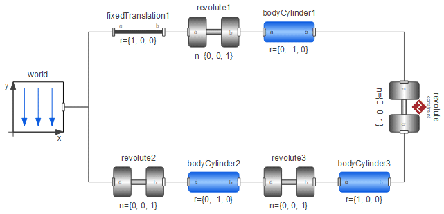
Modelica.MultiBody is a Modelica library for 3D mechanical modeling. Working with 3D models can be complicated, since all parts need to be connected in space and initial values need to be correct in order for the system to start. System Modeler contains visualization for models created with the MultiBody library to aid the user in analyzing the movement in a convenient way. Following are some important things to consider when working with the MultiBody library. An introduction to the library as well as information about its components can be found by accessing the embedded documentation of the Modelica.MultiBody package and its classes. The following figure shows a model of a planar loop built with the MultiBody library.

Initial Values
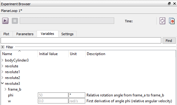
It is important to get the system to initialize the states properly to get a physically correct model. In this example, we have chosen to use the states in the revolute3 component by setting the parameter stateSelect in revolute3 to StateSelect.always. When the model is translated or built, appropriate states are selected. The initial values of these states are shown in the Variables tab in Simulation Center.

Selected states for the model in the previous screen shot.
As seen in the preceding screen shot, the angle of the joint revolute3 will start with the speed 0.0 rad/s and at the angle 50 degrees. These values can also be changed directly in the model in the General tab in Model Center.
Angle and Position of Objects
It is very important to get a physically correct model, otherwise the system will likely fail to start a simulation. Try to use simple directions, e.g. r={1,0,0}, r={0,-1,0} for components like BodyCylinder, BodyBox, etc. If another direction is needed, change phi in a joint or use the FixedRotation and FixedTranslation components available in MultiBody.Parts.
Animations
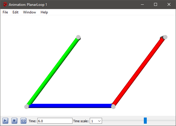
Some of the MultiBody components contain animation information. These are the Body, BodyBox, BodyCylinder, and BodyShape components in MultiBody.Parts. There are also visualizers that show properties like velocity, acceleration, etc. in MultiBody.Visualizers.

Animation of a simple loop model containing three bars from the preceding model.
As indicated by their respective names, the BodyBox is box shaped and the BodyCylinder is cylinder shaped. If more variants of animated shapes are needed, e.g. sphere, cone, gearwheel, etc., the BodyShape can be used, setting the parameter shapeType to the desired shape. If only a pure animation is needed without physical properties, the Shape object can be used.
The following figure shows an example of a pendulum with a sphere at the end, where the BodyShape component has been used to animate the sphere. The visualization of the pendulum model can be seen at the far right.

A pendulum model with a sphere shape at the end.
CAD Shapes
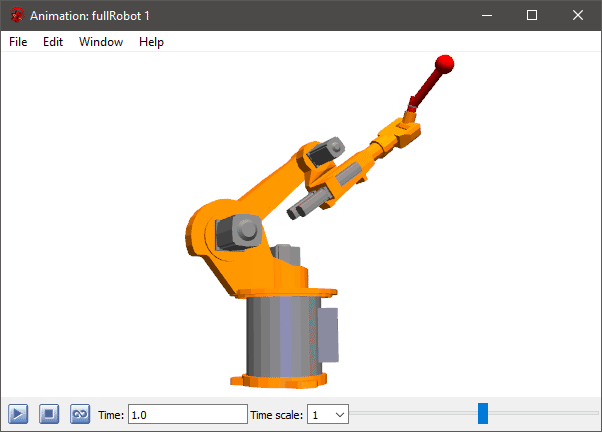
CAD shapes are specified by setting the shapeType parameter to a Modelica URI that points to the CAD file. A Modelica URI has the following structure:
modelica://<Modelica-name>/<relative-file-path>
This specifies the path ![]() relative to the location of the Modelica library <Modelica-name>.
relative to the location of the Modelica library <Modelica-name>.
System Modeler supports the following CAD shape formats:

Animation view of Modelica.Mechanics.MultiBody.Examples.Systems.RobotR3.fullRobot.
General Advice
Following is a collection of general tips that may prove useful to avoid some common problems.
- Debugging equation-based languages is a different task compared to algorithm-based languages, since it is not possible to add break points, solve step by step, etc. Therefore, try to build up your model step by step, i.e. make small tests of partial systems of your complete model. If an error occurs, it will be a lot easier to locate if the model is small.
- Use the Validate Class feature, described here, when creating components. If a component validation is successful, it is more likely that the component will work together with other components. A complete component should always return an equal number of variables and equations from the validation. Note that a partial model naturally often returns a different number of equations than variables.
- If a simulation takes a long time, it could be due to a large number of events. The number of events can be found in the simulation log after a simulation is finished. If possible, try to reduce the number of events by using the noEvent operator (see preceding explanation) or try to change your model. Note that when modeling sampled systems, an event is generated at each sample time, which is normal.
- Try to avoid the automatic setting of output intervals when simulating a well-known system. Since data is written to file at each solver step, this could drastically reduce the simulation performance for larger systems. When the model behavior is known, it is recommended to switch to a fixed number of output intervals or use an interval length setting instead.
