This guide gives a short introduction to the Wolfram Hydraulic library, which consists of components for modeling and simulating hydraulic systems. Here you will learn how to use the library to build hydraulic circuits with predefined components, such as pumps and motors, cylinders, valves, and specialized hydraulic ports, but also how to create your own customized components.

The design idea behind the Hydraulic library was to create a general purpose Modelica library for modeling, simulating, and visualizing hydraulic systems, as well as to create a library connectable with libraries in other domains such as automotive and aerospace. As an example, the pumps and motors in Hydraulic can be connected to rotational mechanical components from the Modelica Standard Library.

Building Your First Model

In this first example we will implement a hydraulic circuit with an unloading relief valve and an accumulator. The idea behind this model is to show how an unloading relief valve can be used to limit the maximum pressure in a hydraulic circuit when a certain desired accumulator pressure has been reached.

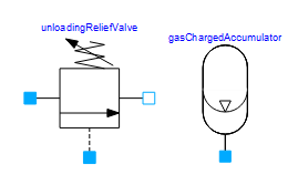
The main components of the hydraulic circuit will be the UnloadingReliefValve and the GasChargedAccumulator.

Creating a New Model in Wolfram SystemModeler

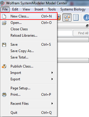
Creating a new model in Wolfram SystemModeler.

The first step is to create a new model. This is done by choosing File ▶ Class, as illustrated in the screenshot above. This will open a dialog box in which different model properties, such as model name and description, can be specified. A short description of the model is recommended to keep track of the modeling work. After clicking OK, a new model will be created and its (empty) diagram view will be opened.

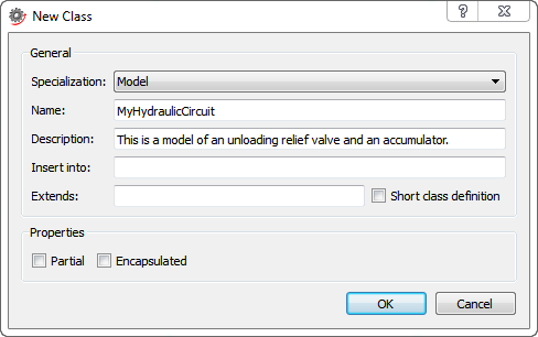
Creating a new model named MyHydraulicCircuit.

Adding the Main Components

The next natural step is to add the main components that will be needed in the hydraulic circuit, i.e the relief valve and the accumulator. In this case, a component named GasChargedAccumulator, found in package Hydraulic.LiquidContainers, will be used as the accumulator in the circuit. This package also contains other types of containers, such as tanks and volumes with fixed storage.

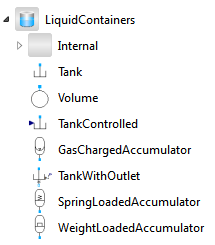
Finding the GasChargedAccumulator component in the Class Browser.

The valve component is named UnloadingReliefValve and can be found in package Hydraulic.Valves.PressureControl.

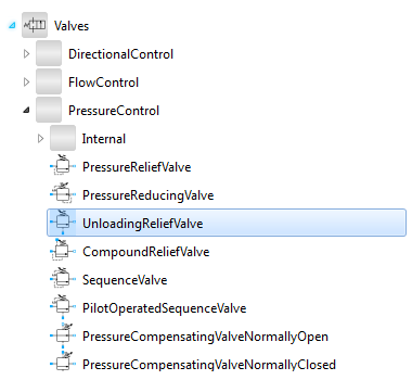
Finding the UnloadingReliefValve component in the Class Browser.

After locating the components in the Libraries section of the Class Browser, adding them to the model is a simple matter of dragging and dropping the components onto the diagram view. This creates instances of the two models, namely gasChargedAccumulator and unloadingReliefValve.

Clicking on the valve component once enables a view in the bottom window in which component-specific parameters can be viewed and modified. The tabs General and Geometries contain parameters for e.g port leakage, pressure, and volume. The accumulator component has one additional tab, named Initialization, where initial values for accumulator volume, pressure, and gas volume can be specified. All these values can be modified to fit the system currently being modeled.

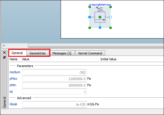
Clicking the valve component enables a view where general properties, such as medium and pressure limits and component geometries, can be modified.

Adding the Remaining Components

The time has come to start adding the other components needed to create the hydraulic circuit. For this example the following hydraulic components will be used:

• Hydraulic.LiquidContainers.Tank
• Hydraulic.PumpsAndMotors.Pump
• Hydraulic.Valves.DirectionalControl.CheckValve
• Hydraulic.Valves.FlowControl.FixedLaminarThrottle

In addition, a rotational component named ConstantSpeed, found in package Modelica.Mechanics.Rotational.Sources, will be used. By connecting this component to the pump it will keep the pump's angular velocity constant.

The component CheckValve is introduced to prevent reverse fluid flow from the accumulator, and so it needs to be connected to the pump and relief valve on one side and to the accumulator part of the circuit on the other side.

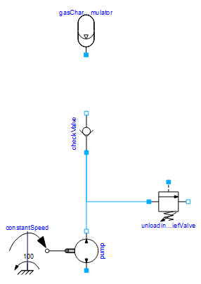
At this stage, the hydraulic circuit contains a hydraulic pump connected to a rotational component with constant speed. The pump and relief valve have both been connected to the check valve in order to prevent reverse flow from the accumulator.

In a real hydraulic circuit the accumulator would most likely be connected to some system, for example a brake system, for which it can provide a source of reserve power. In this example, we'll let the system be represented by a fixed laminar throttle valve and a tank. The throttle valve controls the flow by laminar restriction and since it affects the flow it also affects the pressure in the hydraulic circuit. The throttle valve will be connected to a tank on one side and to the accumulator, check valve, and relief valve on the other side. This will have the effect of putting a load on the circuit.

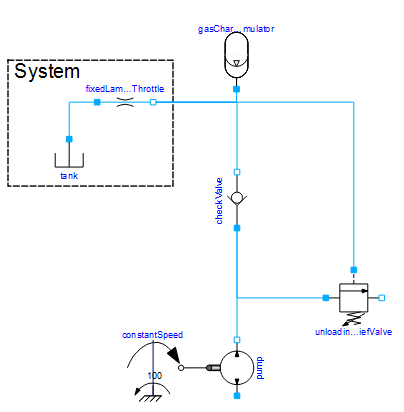
A load in the form of a tank and a throttle valve has been put on the hydraulic circuit.

The tanks have unlimited volume and can be used as sinks or sources of medium. We need two additional tanks, one that connects to the pump and one that connects to port_a in the unloading relief valve. Adding these two tanks completes the hydraulic circuit we set out to build.

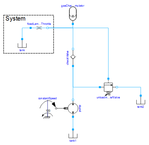
The complete hydraulic circuit.

Simulating the Model

The model is now ready for simulation. However, at this point all parameters and initial values for variables still have their default values and there are no explicit experiment settings for the model. It is of course possible to simulate with the default settings for both parameter values and experiment settings, but in this case we would like to introduce some modifications. All default values for parameters and variables are kept except for the valve parameters pMax and pMin, which decide at what pressure the valve is fully open and when it starts to open, respectively. Let's set these to 3.1 MPa and 3.0 MPa.

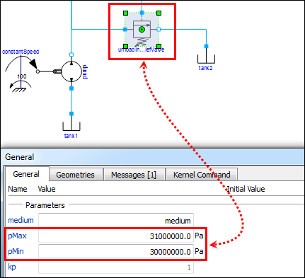
Modified values for parameters pMax and pMin in the unloading relief valve.

The simulation stop time is also set to 1 s instead of the default setting of 10 s. The experiment settings can be changed by pressing the down button next to the Simulate Class icon and choose Experiment Setup. This will open up the Class Properties dialog in which all experiment settings can be adjusted.

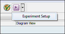
To change experiment settings, choose Experiment Setup from the toolbar.

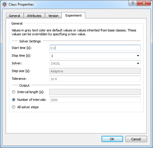
The experiment settings can be modified from the Class Properties window.

Clicking the Simulate Class button in the toolbar will simulate the model and open Simulation Center. In Simulation Center it is possible to plot any parameter or variable, for example accumulator pressure or the mass flow through the relief valve. This screenshot shows a plot of these two variables.

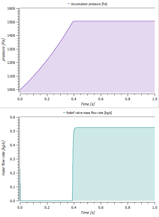
Plot of the accumulator pressure and the mass flow rate through the relief valve in a 1 s simulation.

The uppermost plot shows how the pressure in the accumulator builds up until the pressure limit of 15×10⁶ Pa is reached. The time the limit is reached is also the time when the mass flow rate through the relief valve starts to grow rapidly (bottom plot) to unload the pump and limit the accumulator pressure.

Building Custom Components

The Wolfram Hydraulic library contains more than 200 ready-made classes, some of which have already been introduced in the previous sections. However, sometimes there might be a necessity to create a customized and reusable component to better suit the current modeling needs. An example of such a component could, for example, be a hydraulic motor component with capabilities for predicting heat generation and power loss. Let's call this new model MotorWithLoss.

Building a New Component

In creating MotorWithLoss, it is most timesaving to use the built-in component Motor found in package Hydraulic.PumpsAndMotors and extend from it in the new model. Also, it is convenient to be able to connect the motor power loss and heat generation to other components when used in a larger system. Therefore the new model will also extend from the partial model Modelica.Thermal.HeatTransfer.Interfaces.PartialElementaryConditionalHeatPortWithoutT.

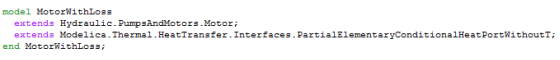
MotorWithLoss extending from two other models, one from Hydraulic and one from the Modelica Standard Library.

Extending from these models, MotorWithLoss automatically obtains an icon and a diagram layer with the components inherited from the extended classes.

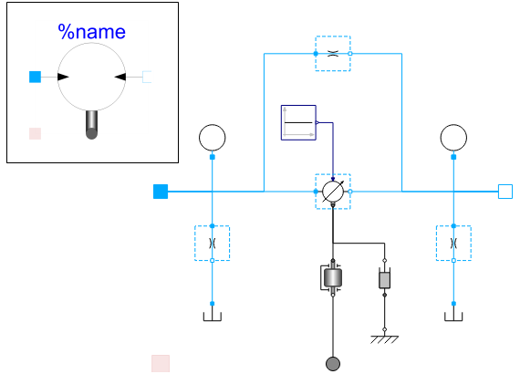
The image shows the diagram view of MotorWithLoss. The top-left corner shows the icon.

The next step is to add the equations needed to describe the power loss in the motor. This loss is represented by variable lossPower, which is available in MotorWithLoss through the heritage from PartialElementaryConditionalHeatPortWithoutT. The required power equations are:

where p pressure [Pa], Q volumetric flow [m³/s], τ torque [Nm], ω angular velocity [rad/s], P_f fluid power and P_m mechanical rotational power.

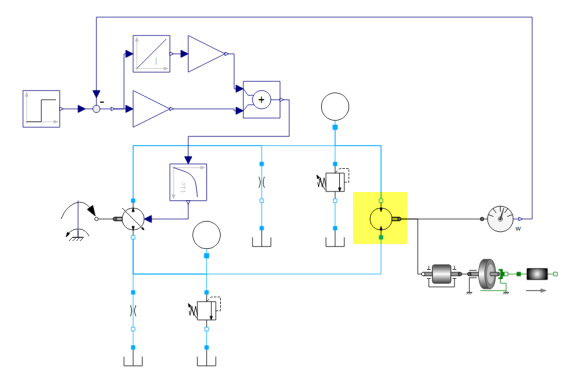
Examining the diagram view, it becomes apparent that there are three power sinks and sources that need to be taken into account; the fluid power at port_a and port_b and the mechanical power transferred through the flange.

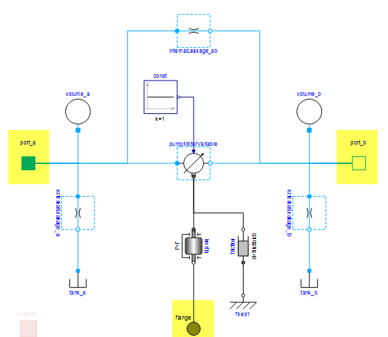
MotorWithLoss in the diagram view in SystemModeler. The needed power sinks and sources are highlighted in yellow.

The ports and the flange already contain variables for pressure, flow, torque, and angular velocity, but the flow needs to be converted from mass flow to volumetric flow. Let's create two new variables, volumetricFlow_a and volumetricFlow_b, and use the unit for VolumeFlowRate available in package Modelica.Units.SI. Dividing the mass flow with the density of the medium, medium.rho, yields the volumetric flow.

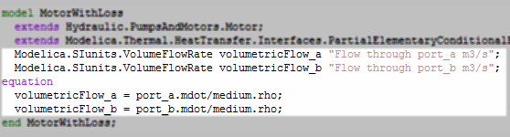
The MotorWithLoss model with the newly added variables and equations. Adding short comments to all parameters, constants, and variables in a model is a good way to keep track of the modeling work and makes it easier for others to follow.

Now everything needed to calculate the power loss is readily available. Let's introduce five new variables to wrap it all together:

• power_a, power_b: the power at port a and b, respectively
• absPowerOut: a variable for the absolute value of the power released by the motor through the flange
• powerDiff: the power difference between port a and b
• checkSum: a control variable to easily be able to check that the sum of all powers is 0

Not all five variables are absolutely necessary for the model to work, but they make it easier to analyze the simulation results. The equations that need to be translated into Modelica code are then:

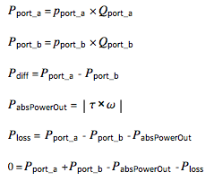
Note that some equations in the model below have different signs compared to the equations just given. This is because certain variables, such as power_a and power_b, take on positive or negative values depending on the direction of flow.

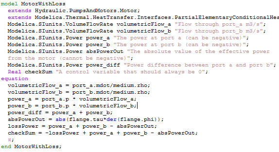
The final model.

So now that the component is ready, let's incorporate it into a larger model.

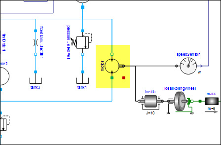
A hydraulic circuit with the MotorWithLoss component highlighted in yellow.

The model above is a hydraulic circuit in which a pump drives the hydraulic motor (highlighted in yellow). The circuit is a hydrostatic transmission that has a feedback loop that controls the angular velocity of the motor by changing the pump displacement. Three additional components (inertia, idealRollingWheel, and mass) have been connected to the motor to function as a load. The plots below show the custom characteristics of the MotorWithLoss component.

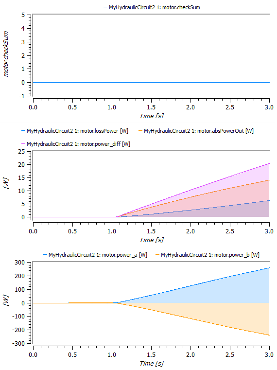
The uppermost plot shows the checkSum variable, which as expected remains at 0 during the simulation. The middle plot shows how much fluid power that in theory could be turned into rotational power (power_diff), how much is actually being turned into mechanical power (absPowerOut), and finally how much is lost to the environment (lossPower). The bottom plot shows the power at port_a and port_a, at which the power is either positive or negative depending on if the flow is directed into the port or out of the port.

As previously mentioned, the heritage from PartialElementaryConditionalHeatPortWithoutT makes it possible to connect the power loss and heat generation to other components, for example a convection element. This is done by changing the inherited parameter useHeatPort from false to true. That will make a red connector visible, which can be connected to other thermal models.

Setting useHeatPort to true enables a heat port marked in red. The motor component, together with its enabled heat port, is highlighted in yellow in the image.

After this getting started guide on how to create some simpler models using Wolfram Hydraulic, you should now be able to continue on your own and further explore the capabilities of the library.