WOLFRAM SYSTEM MODELER
OverViewOverview of MultiBody library |
|
Wolfram Language
In[1]:=
SystemModel["Modelica.Mechanics.MultiBody.UsersGuide.Tutorial.OverView"]
Out[1]:=
Information
This information is part of the Modelica Standard Library maintained by the Modelica Association.
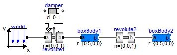
Library MultiBody is a free Modelica package providing 3-dimensional mechanical components to model in a convenient way mechanical systems, such as robots, mechanisms, vehicles. A basic feature is that all components have animation information with appropriate default sizes and colors. A typical screenshot of the animation of a double pendulum is shown in the figure below, together with its schematic.
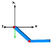
Note, that all components - the coordinate system of the world frame,
the gravity acceleration vector, the revolute joints and the
bodies - are visualized in the animation.
This library replaces the long available ModelicaAdditions.MultiBody
library, since it is much more easier to use and more powerful.
The main features of the library are:
- About 60 main components, i.e., joint, force, part, body, sensor and visualizer components that are ready to use and have useful default animation properties. One-dimensional force laws can be defined with components of the Modelica.Mechanics.Rotational and of the Modelica.Mechanics.Translational library and can be connected via available flange connectors to MultiBody components.
- About 75 functions to operate in a convenient way on orientation objects, e.g., to transform vector quantities between frames, or compute the orientation object of a planar rotation. The basic idea is to hide the actual definition of an orientation by providing essentially an Orientation type together with functions operating on instances of this type. Orientation objects based on a 3x3 transformation matrix and on quaternions are provided. As a side effect, the equations in all other components are simpler and easier to understand.
- A World model has to be present in every model on top level. Here the gravity field is defined (currently: no gravity, uniform gravity, point gravity), the visualization of the world coordinate system and default settings for animation. If a world model is not present, it is automatically provided together with a warning message.
- Built-in animation properties of all components, such as joints, forces, bodies, sensors. This allows an easy visual check of the constructed model. Animation of every component can be switched off via a parameter. The animation of a complete system can be switched off via one parameter in the world model. If animation is switched off, all equations related to animation are removed from the generated code. This is especially important for real-time simulation.
- Automatic handling of kinematic loops. Components can be connected together in a nearly arbitrary fashion. It does not matter whether components are flipped. This does not influence the efficiency. If kinematic loop structures occur, this is automatically handled in an efficient way by a new technique to transform a certain class of overdetermined sets of differential algebraic equations symbolically to a system where the number of equations and unknowns are the same (the user need not cut loops with special cut-joints to construct a tree-structure).
- Automatic state selection from joints and bodies. Most joints and all bodies have potential states. A Modelica translator will use the generalized coordinates of joints as states if possible. If this is not possible, states are selected from body coordinates. As a consequence, strange joints with 6 degrees of freedom are not necessary to define a body moving freely in space. An advanced user may select states manually from the Advanced menu of the corresponding components or use a Modelica parameter modification to set the "stateSelect" attribute directly.
- Analytic solution of kinematic loops. The non-linear equations occurring in kinematic loops are solved analytically for a large class of mechanisms, such as a 4 bar mechanism, a slider-crank mechanism or a MacPherson suspension. This is performed by constructing such loops with assembly joints JointXXX, available in the Modelica.Mechanics.MultiBody.Joints package. Assembly joints consist of 3 joints that have together 6 degrees of freedom, i.e., no constraints.They do not have potential states. When the motion of the two frame connectors are provided, a non-linear system of equation is solved analytically to compute the motion of the 3 joints. Analytic loop handling is especially important for real-time simulation.
- Line force components may have mass. Masses of line force components are located on the line on which the force is acting. They approximate the mass properties of a real physical device by one or two point masses. For example, a spring has often significant mass that has to be taken into account. If masses are set to zero, the additional code to handle these point masses is removed. If the masses are taken into account, the calculation overhead is small (the reason is that the occurring kinematic loops are analytically solved).
- Force components may be connected directly together, e.g., 3-dimensional springs in series connection. Usually, multi-body programs have the restriction that force components can only be connected between two bodies. Such restrictions are not present in the Modelica multi-body library, since it is a fully object-oriented, equation based library. Usually, if force components are connected directly together, non-linear systems of equations occur. The advantage is often, that this may avoid stiff systems that would occur if a small mass has to be put in between the two force elements.
- Initialization definition is available via menus. Initialization of states in joints and bodies can be performed in the parameter menu, without typing Modelica statements. For non-standard initialization, the usual Modelica commands can be used.
- Multi-body specific error messages. Annotations and assert statements have been introduced that provide in many cases warning or error messages that are related to the library components (and not to specific equations as it is usual in Modelica libraries). This requires appropriate tool support, as it is.
- Inverse models of mechanical systems can be easily defined by using motion generators, e.g., Modelica.Mechanics.Rotational.Position. Also, non-standard inverse models can be generated, e.g., when elasticity is present it might be necessary to differentiate equations several times.