Solving Partial Differential Equations with Finite Elements
| Introduction | Classical Partial Differential Equations |
| Regions | Systems of Partial Differential Equations |
Introduction
The aim of this tutorial is to give an introductory overview of the finite element method (FEM) as it is implemented in NDSolve. The notebook introduces finite element method concepts for solving partial differential equations (PDEs). First, typical workflows are discussed. The setup of regions, boundary conditions and equations is followed by the solution of the PDE with NDSolve. The visualization and animation of the solution is then introduced, and some theoretical aspects of the finite element method are presented. Classical PDEs such as the Poisson and Heat equations are discussed. Coupled PDEs are also introduced with examples from structural mechanics and fluid dynamics.
Why Finite Elements?
Explicit closed-form solutions for partial differential equations (PDEs) are rarely available. The finite element method (FEM) is a technique to solve partial differential equations numerically. It is important for at least two reasons. First, the FEM is able to solve PDEs on almost any arbitrarily shaped region. Second, the method is well suited for use on a large class of PDEs. While it is almost always possible to conceive better methods for a specific PDE on a specific region, the finite element method performs quite well for a large class of PDEs. In summary, the finite element method is important since it can deal with:
What Is Needed for a Finite Element Analysis
To solve partial differential equations with the finite element method, three components are needed:
This section deals with partial differential equations and their boundary conditions. Finite element meshes can be generated with ToElementMesh. A tutorial on the generation of finite element meshes can be found in "Element Mesh Generation".
The Scope of the Finite Element Method as Implemented in NDSolve
The current version of the implementation of the finite element method supports the following features:
- linear variable coefficient Dirichlet conditions; generalized, possibly nonlinear, Neumann (Robin) boundary values; and a mixture of these boundary conditions are possible
The following sections provide an overview of this functionality. For an extended list of what PDEs can be solved, please also consult the PDE Models Overview page or the PDEModeling guide page for a specific field of physics and engineering.
For convenient use of the finite element functionality, load the finite element package.
Needs["NDSolve`FEM`"]Regions
To perform a finite element analysis, a region over which the partial differential equation is to be solved needs to be defined. Rectangular regions may be specified using {v,vmin,vmax} for each of the spatial independent variables. The exact argument specification is detailed in NDSolveValue.
ufun = NDSolveValue[{-Laplacian[u[x, y], {x, y}] == 10,
	u[x, 0] == 0, u[x, 1] == 1},
	u, {x, 0, 1}, {y, 0, 1}];
Plot3D[ufun[x, y], {x, 0, 1}, {y, 0, 1}, ColorFunction -> "TemperatureMap"]
Regions of arbitrary shape may be specified using the notation vars∈Ω, where Ω is a region so that RegionQ[Ω] gives True.
One way to specify a nonrectangular region is by using Boolean predicates. A predicate is a function that returns either True or False. Since the term predicate has many meanings in mathematical literature, the terminology Boolean predicate is used to emphasize that the predicate returns a Boolean. To describe regions, Boolean predicates can be used as in functions like RegionPlot and RegionPlot3D, for example.
Ω = ImplicitRegion[!((x - 5) ^ 2 + (y - 5) ^ 2 ≤ 3 ^ 2), {{x, 0, 5}, {y, 0, 10}}];
RegionPlot[Ω, AspectRatio -> Automatic]
This tutorial concentrates on solving partial differential equations with the finite element method, without emphasis on the creation of regions and meshes. More detailed information on this topic can be found in "Element Mesh Generation".
Classical Partial Differential Equations
The Coefficient Form of Partial Differential Equations
What types of equations can be solved with the finite element method as implemented in NDSolve? Consider a single partial differential equation in ![]() :
:
The PDE is defined in ![]() . Here
. Here ![]() is the dependent variable for which a solution is sought. The coefficients
is the dependent variable for which a solution is sought. The coefficients ![]() ,
, ![]() ,
, ![]() and
and ![]() are scalars;
are scalars; ![]() ,
, ![]() and
and ![]() are vectors; and
are vectors; and ![]() is an
is an ![]() ×
×![]() matrix.
matrix.
What follows are some well-known PDEs and their corresponding coefficients. To illustrate the generality of (1), the components that are relevant to a specific equation are red, while the non-relevant components are grayed out.
The Laplace equation simply contains a diffusive term:
To model Poisson's equation, only a small modification is needed; add a load term ![]() :
:
Helmholtz's equation adds a reaction term ![]() :
:
Convection-diffusion-reaction type equations are another common class of PDEs. Compared to the previous examples, these have an additional convection term ![]() :
:
The PDEs considered so far are stationary, i.e. they have no time dependence. The heat equation adds time dependence to the Poisson equation. It has the following form:
Similarly, the wave equation is given as:
Equation (1) provides the components for modeling a range of different phenomena, since it provides spatial derivatives up to order 2.
Poisson’s Equation with Dirichlet Conditions
The Poisson equation is to be solved over a region ![]() with boundary conditions. First, a region needs to be defined where the equation will be solved. Then the equation and boundary conditions are defined. Finally, the equation is solved over the region.
with boundary conditions. First, a region needs to be defined where the equation will be solved. Then the equation and boundary conditions are defined. Finally, the equation is solved over the region.
One way to specify a region is by using Boolean predicates.
Ω = ImplicitRegion[!((x - 5) ^ 2 + (y - 5) ^ 2 ≤ 3 ^ 2), {{x, 0, 5}, {y, 0, 10}}];
RegionPlot[Ω, AspectRatio -> Automatic]
Next, define a Poisson operator.
op = -Laplacian[u[x, y], {x, y}] - 20;The third step is to set up the boundary conditions. The first boundary condition enforces the dependent variable ![]() to a value of 0 wherever the evaluation of x0∧8≤y≤10 yields True on the boundary of the region
to a value of 0 wherever the evaluation of x0∧8≤y≤10 yields True on the boundary of the region ![]() . In this case, this is the upper-left part of the boundary. This type of boundary condition is called a Dirichlet boundary condition. A second Dirichlet boundary condition specifies the value of the dependent variable
. In this case, this is the upper-left part of the boundary. This type of boundary condition is called a Dirichlet boundary condition. A second Dirichlet boundary condition specifies the value of the dependent variable ![]() whenever
whenever ![]() yields True on the boundary of region
yields True on the boundary of region ![]() . Boundary conditions will be explained in further detail in a later section.
. Boundary conditions will be explained in further detail in a later section.
Subscript[Γ, D] = {DirichletCondition[u[x, y] == 0, x == 0 && 8 ≤ y ≤ 10],
	DirichletCondition[u[x, y] == 100, (x - 5) ^ 2 + (y - 5) ^ 2 == 3 ^ 2]};
In the solution step, NDSolve needs the PDE, the boundary conditions and the region.
ufun = NDSolveValue[{op == 0, Subscript[Γ, D]}, u, {x, y}∈Ω]Internally, the region ![]() is converted to a finite element mesh and a finite element method is used to solve the equation automatically.
is converted to a finite element mesh and a finite element method is used to solve the equation automatically.
To visualize the solution, a contour plot can be used.
ContourPlot[ufun[x, y], {x, y}∈Ω, ColorFunction -> "Temperature", AspectRatio -> Automatic]Partial Differential Equations and Boundary Conditions
NDSolve and related functions allow for specifying three types of spatial boundary conditions: Dirichlet conditions, Neumann values and periodic boundary conditions.
Dirichlet boundary conditions prescribe a constraint on the dependent variable ![]() of value
of value ![]() on some part of the boundary:
on some part of the boundary:
Generalized Neumann boundary values, also known as Robin values or Neumann boundary conditions, specify a value ![]() . The value
. The value ![]() prescribes a flux over the outward normal on some part of the boundary:
prescribes a flux over the outward normal on some part of the boundary:
The finite element method is based on the weak form of the differential equation. This form is obtained by taking equation (1), multiplying it by a so-called test function ![]() , and integrating over the region
, and integrating over the region ![]() :
:
This process is done internally. The integrand in the boundary integral in (11) ![]() can be replaced with
can be replaced with ![]() (9) and yields:
(9) and yields:
![]() specifies the value of the boundary integral integrand (11) in the weak form and thus the name NeumannValue.
specifies the value of the boundary integral integrand (11) in the weak form and thus the name NeumannValue.
Instead of making use of integration by parts to obtain equation (11), the divergence theorem and Green's identities can also be used.
Periodic boundary conditions make the dependent variables behave according to a given relation between two distinct parts of the boundary. Other boundary conditions are conceivable, but currently not implemented.
In most cases, Dirichlet boundary conditions need not be associated with a particular equation. They can be specified independently of the equation. Dirichlet boundary conditions are specified as equations. Generalized Neumann values, on the other hand, are specified by giving a value, since the equation satisfied is implicit in the value. Neumann values are mathematically tied to the PDE.
For practical reasons, in NDSolve and related functions, NeumannValue needs to be given as a part of the equation. Consider a system of coupled PDEs. One would like to be able to unambiguously specify any given Neumann value to any given single PDE of that system of PDEs. It is not possible to derive (unambiguously) from the Neumann value with which PDE equation the value should be associated. Making a NeumannValue part of a PDE equation solves this problem without ambiguity. DirichletCondition may also be given in a PDE equation as well.
| {op[u[x1,…]] ΓN,ΓD,ΓP} | partial differential equation with differential operator op, Neumann boundary values ΓN, Dirichlet boundary condition equations ΓD and periodic boundary condition ΓP |
| {op1[u[x1,…],v[x1,…],…] ΓN1,op2[u[x1,…],v[x1,…],…] ΓN2,…,ΓD,ΓP} | system of coupled partial differential equation operators opj, Neumann boundary values ΓNj and Dirichlet and periodic boundary condition equations ΓD and ΓP |
Specifying partial differential equations with boundary conditions.
DirichletCondition, NeumannValue and PeriodicBoundaryCondition all require a second argument that is a predicate describing the location on the boundary where the conditions/values are to be applied. Additionally, the PeriodicBoundaryCondition has a third argument specifying the relation between the two parts of the boundary.
A partial differential equation typically needs at least one Dirichlet boundary condition on some part of the region to be uniquely solvable. For this reason, Dirichlet boundary conditions are also called essential boundary conditions.
The use of generalized Neumann values arises from the boundary integral from the weak form, and so they are also commonly referred to as natural conditions.
A pure Neumann boundary equation is a generalized Neumann boundary equation (9) where ![]() :
:
If ![]() is also not specified, then a Neumann zero boundary value is automatically implied (
is also not specified, then a Neumann zero boundary value is automatically implied (![]() ):
):
Note that when the Neumann value is zero, the term drops out in (12). This is typically a case where there is no flux or stress at the boundary. When no boundary conditions are explicitly specified for a part of the region boundary ![]() , a Neumann zero value is assumed.
, a Neumann zero value is assumed.
Poisson’s Equation with Neumann Values
Consider the solution of Poisson's equation with generalized Neumann boundary values.
Ω = ImplicitRegion[!((x - 5) ^ 2 + (y - 5) ^ 2 ≤ 3 ^ 2), {{x, 0, 5}, {y, 0, 10}}];
op = -Laplacian[u[x, y], {x, y}] - 20;
Poisson's equation is given as:
The corresponding Neumann boundary equation is:
Note how the normal derivative of the Neumann-type equation relates to the PDE. In the Neumann boundary equation, one specifies the values of ![]() and
and ![]() on the right-hand side. The left-hand side is implicitly specified through the PDE. If the coefficient
on the right-hand side. The left-hand side is implicitly specified through the PDE. If the coefficient ![]() in the PDE is given as an identity matrix, then the coefficient
in the PDE is given as an identity matrix, then the coefficient ![]() on the left-hand side of the Neumann equation is that same coefficient
on the left-hand side of the Neumann equation is that same coefficient ![]() .
.
The Neumann boundary value is specified though the values ![]() and
and ![]() . Typically when
. Typically when ![]() , one speaks of a Neumann boundary value, and in the case
, one speaks of a Neumann boundary value, and in the case ![]() , one speaks of a generalized Neumann or Robin boundary value. It is common to use the term Neumann boundary condition for both the generalized Neumann and Neumann boundary value.
, one speaks of a generalized Neumann or Robin boundary value. It is common to use the term Neumann boundary condition for both the generalized Neumann and Neumann boundary value.
Subscript[Γ, N] = NeumannValue[-2u[x, y], ((x - 5) ^ 2 + (y - 5) ^ 2 == 3 ^ 2)];Subscript[Γ, D] = DirichletCondition[u[x, y] == 0, x == 0 && 8 ≤ y ≤ 10];It is important to observe that the constants in the term ![]() of the Neumann boundary equation exactly match the constants in
of the Neumann boundary equation exactly match the constants in ![]() from the weak form of the PDE (11). Because these terms are required to match, NeumannValue only requires the user to enter the right-hand side of the boundary equation. For example, to enter the boundary equation
from the weak form of the PDE (11). Because these terms are required to match, NeumannValue only requires the user to enter the right-hand side of the boundary equation. For example, to enter the boundary equation ![]() , it suffices to enter NeumannValue[1,…]. The correct expression for the left-hand side of the boundary equation (i.e.
, it suffices to enter NeumannValue[1,…]. The correct expression for the left-hand side of the boundary equation (i.e. ![]() ) is implied by the term
) is implied by the term ![]() in the weak form of the PDE (12). This close relation of the Neumann boundary value and the PDE is further accommodated by making the NeumannValue part of the equation.
in the weak form of the PDE (12). This close relation of the Neumann boundary value and the PDE is further accommodated by making the NeumannValue part of the equation.
ufun = NDSolveValue[{op == Subscript[Γ, N], Subscript[Γ, D]}, u, {x, y}∈Ω]Plot3D[ufun[x, y], {x, y}∈Ω]In the previous examples, not all boundaries had boundary conditions explicitly attributed; for those parts of the boundaries, the Neumann zero condition is used.
Plot[ufun[0, y], {y, 0, 10}]Note that the values beyond 8 are zero, as required by the Dirichlet condition.
Poisson’s Equation with a Periodic Boundary Condition
The purpose of PeriodicBoundaryCondition is to relate the values of a solution of a PDE at two distinct parts of the boundary. PeriodicBoundaryCondition[a+b u,pred,f] specifies a periodic boundary condition where the predicate pred specifies a target at which the solution should relate to values from a distinct source, and the function f maps coordinates from the target locations (blue) to the source locations (green) where the dependent variable relation is evaluated. The resulting values will be set as a condition at the target.

An example is the best way to understand how PeriodicBoundaryCondition works.
Ω = ImplicitRegion[1 ≤ x ^ 2 + y ^ 2 ≤ 2 ^ 2 && x - y ≥ 0 && x ≥ 0 && y ≥ 0, {x, y}];
Show[
	RegionPlot[Ω],
	ContourPlot[y - x == 0, {x, 1 / Sqrt[2], 2}, {y, -0.1, Sqrt[2]}, ContourStyle -> Blue],
	ContourPlot[y == 0, {x, 1, 2}, {y, -0.1, Sqrt[2]}, ContourStyle -> Green], AspectRatio -> Automatic]
The PDE in this example is a Laplacian with a load term of 1 unit active in a rectangle specified by ![]() . Everywhere else there the load is 0.
. Everywhere else there the load is 0.
pde = -Laplacian[u[x, y], {x, y}] == If[1.4 ≤ x ≤ 1.6 && 0 ≤ y ≤ 0.1, 1, 0];PeriodicBoundaryCondition allows either periodic or antiperiodic or relational boundary conditions to be modeled. In this example, a periodic boundary condition is presented. A periodic condition is specified when the first argument is the dependent variable, u, and requires that the dependent variable u at the predicate ![]() (blue, target) is to have the same values as at position
(blue, target) is to have the same values as at position ![]() (green, source). During the solution process, the dependent variable u is to be evaluated at the source. For this, a mapping from the predicate
(green, source). During the solution process, the dependent variable u is to be evaluated at the source. For this, a mapping from the predicate ![]() (blue, target) to
(blue, target) to ![]() (green, source) is needed. The function FindGeometricTransform can construct such a mapping from a list of coordinates.
(green, source) is needed. The function FindGeometricTransform can construct such a mapping from a list of coordinates.
mapping = Last[FindGeometricTransform[{{1, 0}, {2, 0}}, {{1 / Sqrt[2], 1 / Sqrt[2]}, {Sqrt[2], Sqrt[2]}}]];Investigate to see that the mapping maps a point from the green source to the blue target.
mapping[{1., 0}]The PeriodicBoundaryCondition is then set up by giving the relation of the dependent variable, the target predicate and a mapping. In the periodic case, the relation is ![]() .
.
Subscript[Γ, P] = PeriodicBoundaryCondition[u[x, y], y - x == 0, mapping];Additionally, on both curved sides DirichletCondition is placed. Note that the DirichletCondition is excluded at ![]() such that there is no DirichletCondition on the target boundary. Having Dirichlet boundary conditions there would not be consistent with the solution mapped to these places.
such that there is no DirichletCondition on the target boundary. Having Dirichlet boundary conditions there would not be consistent with the solution mapped to these places.
Subscript[Γ, D] = DirichletCondition[u[x, y] == 0, (x^2 + y^2 == 1 || x^2 + y^2 == 4) && !(y - x) > -10 ^ -7];ufun = NDSolveValue[{pde, Subscript[Γ, P], Subscript[Γ, D]}, u, {x, y}∈Ω];ContourPlot[ufun[x, y], {x, y}∈Ω, ColorFunction -> "TemperatureMap", AspectRatio -> Automatic]imapping = InverseFunction[mapping];
Plot[{ufun[x, 0] - ufun@@imapping[{x, 0}]}, {x, 1, 2}, PlotRange -> All]An antiperiodic boundary condition can be realized by using the negative of the dependent variable in the PeriodicBoundaryCondition. In the next example, everything except the antiperiodic boundary condition remains the same.
Subscript[Γ, P] = PeriodicBoundaryCondition[-u[x, y], y - x == 0, mapping];ufun = NDSolveValue[{pde, Subscript[Γ, P], Subscript[Γ, D]}, u, {x, y}∈Ω];ContourPlot[ufun[x, y], {x, y}∈Ω, ColorFunction -> "TemperatureMap", AspectRatio -> Automatic]imapping = InverseFunction[mapping];
Plot[{ufun[x, 0] + ufun@@imapping[{x, 0}]}, {x, 1, 2}, PlotRange -> All]Partial Differential Equations with Variable Coefficients
In the following example, the PDE coefficients depend on space and time. Here ![]() indicates the temporal variable and
indicates the temporal variable and ![]() the spatial variables:
the spatial variables:
The example of a shielded microstrip illustrates the effect of variable coefficients. It is an electrostatics application that can be modeled with a Poisson equation where the coefficient ![]() is the relative permittivity
is the relative permittivity ![]() and depends on space:
and depends on space:
A geometry is constructed where the boundary separates two materials. In each material, ![]() has a different value.
has a different value.
First, a boundary mesh is created. For more information about creating element meshes, please consult ToBoundaryMesh.
sh = 2 / 10;sh2 = 2 / 100;sw = 3 / 10;
bmesh = ToBoundaryMesh[
	"Coordinates" -> {{0, 0}, {1, 0}, {1, sh}, {1, 1}, {0, 1}, {0, sh + sh2}, {sw, sh + sh2}, {sw, sh}, {0, sh}},
	"BoundaryElements" -> {LineElement[{{1, 2}, {2, 3}, {3, 4}, {4, 5}, {5, 6}, {6, 7}, {7, 8}, {8, 9}, {9, 1}, {3, 8}}]}
]bmesh["Wireframe"]The conversion of the boundary mesh to an element mesh is done with ToElementMesh.
mesh = ToElementMesh[bmesh];
mesh["Wireframe"]
Next, the PDE is set up. The load term ![]() of the PDE is the charge density
of the PDE is the charge density ![]() divided by the vacuum permittivity
divided by the vacuum permittivity ![]() :
:
The lower part of the geometry ![]() is silicon, while the upper part is vacuum. Silicon has a relative permittivity of about 11.7, while vacuum has a value of 1.
is silicon, while the upper part is vacuum. Silicon has a relative permittivity of about 11.7, while vacuum has a value of 1.
ϵr = If[y ≤ sh, {{11.7, 0.}, {0., 11.7}}, {{1., 0}, {0., 1.}}]Also, see this note about how to set up computationally efficient PDE coefficients.
The charge density ![]() and vacuum permittivity
and vacuum permittivity ![]() are given as follows.
are given as follows.
ρc  = 10 ^ -8.;
ϵ0 = 8.86*^-12;op = Inactive[Div][-ϵr.Inactive[Grad][u[x, y], {x, y}], {x, y}] - ρc / ϵ0For the use of Inactive in PDEs, see the section Formal Partial Differential Equations.
The potential ![]() is set to 0 wherever
is set to 0 wherever ![]() . A second potential is set to 1000 in the inner strip.
. A second potential is set to 1000 in the inner strip.
Subscript[Γ, D] = {DirichletCondition[u[x, y] == 0, x == 1 || y == 1 || y == 0],
DirichletCondition[u[x, y] == 10 ^ 3, 0 ≤ x ≤ sw && sh ≤ y ≤ sh + sh2]};ufun = NDSolveValue[{op == 0, Subscript[Γ, D]}, u, {x, y}∈mesh]Show[ContourPlot[ufun[x, y], {x, y}∈mesh, ColorFunction -> "Temperature"], bmesh["Wireframe"]]In many cases when there are explicit discontinuities in the PDE coefficients, NDSolve automatically includes these in the mesh it generates to solve the problem. The discontinuity at ![]() is automatically detected for this example.
is automatically detected for this example.
sh = 2 / 10;sh2 = 2 / 100;sw = 3 / 10;
Ω = RegionDifference[Rectangle[{0, 0}, {1, 1}], Rectangle[{0, sh}, {sw, sh + sh2}]];
RegionPlot[Ω]ufun = NDSolveValue[{op == 0, Subscript[Γ, D]}, u, {x, y}∈Ω]ToBoundaryMesh[ufun["ElementMesh"]]["Wireframe"]As can be seen, the original input region ![]() did not have an internal boundary at the discontinuity, but during the mesh generation process, the internal line along the discontinuity was added.
did not have an internal boundary at the discontinuity, but during the mesh generation process, the internal line along the discontinuity was added.
An alternative to model multiple materials is to use markers for the specific subregions. This is shown and explained further in the section Markers in the Element Mesh Generation.
Many more multi-material application examples can be found in the application examples of the PDE Models Overview page.
Also, see this note about the setup of efficient PDE coefficients.
Partial Differential Equations with Nonlinear Coefficients
Some PDE coefficients may, in addition to space ![]() and time
and time ![]() , also depend on the dependent variable
, also depend on the dependent variable ![]() and the first derivatives
and the first derivatives ![]() . Here
. Here ![]() indicates the spatial variables
indicates the spatial variables ![]() ,
, ![]() ,
, ![]() . If a coefficient depends on the dependent variable
. If a coefficient depends on the dependent variable ![]() , the equation is nonlinear. Consider the nonlinear equation:
, the equation is nonlinear. Consider the nonlinear equation:
As an example, to compute a minimal surface the following equation can be used:
The equation is nonlinear, since the derivative of the dependent variable appears in the diffusion coefficient.
Ω = Disk[];c = -1 / Sqrt[(1 + Grad[u[x, y], {x, y}].Grad[u[x, y], {x, y}])];
op = Inactive[Div][{{c, 0}, {0, c}} . Inactive[Grad][u[x, y], {x, y}], {x, y}]To solve nonlinear stationary equations, an initial seed for the solution can be specified. This is done by making use of InitialSeeding. InitialSeeding specifies an expression to be evaluated over the region of interest. The expression can depend on the spatial variables. If no initial seed is specified, 0 is assumed as an initial seed.
usol = NDSolveValue[{op == 0, DirichletCondition[u[x, y] == Sin[2π * (x + y)], True]}, u, {x, y}∈Ω]Plot3D[usol[x, y], {x, y}∈Disk[]]More examples on the usage of InitialSeeding can be found on the reference page.
Many more nonlinear application examples can be found in the application examples of the PDE Models Overview page.
Partial Differential Equations with Nonlinear Variable Coefficients
The following section presents a magneto statics application example. Magneto static applications typically make use of several, possibly nonlinear, materials in different areas of the simulation domain. This example looks at a simplified model of a motor, for which the distribution of the magnetic potential and a vector density field of the magnetic flux will be computed.
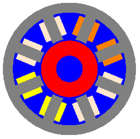
In the preceding representation of the motor geometry, the stator sections are gray, the rotor is red, and the blue area represents air. Also, several coils are grouped and displayed in orange, light orange and yellow.
The PDE model is derived from Ampère's circuital law of Maxwell equations:
Here ![]() is the current density and
is the current density and ![]() the permeability. The magnetic flux density
the permeability. The magnetic flux density ![]() is connected to the magnetic potential
is connected to the magnetic potential ![]() via
via
To simplify the model to two dimensions, assume that currents only flow orthogonal to the ![]() and
and ![]() plane:
plane: ![]() . Further assuming that
. Further assuming that ![]() is constant in the
is constant in the ![]() direction and
direction and ![]() and
and ![]() are constant, you can write:
are constant, you can write:
Since a model is assumed that is homogenous in the ![]() direction, the
direction, the ![]() components drop out and the following is used:
components drop out and the following is used:
The equation is nonlinear, since the permeability ![]() is a function of the spatial coordinates
is a function of the spatial coordinates ![]() and the derivative of the unknown
and the derivative of the unknown ![]() . In the rotor and stator, the permeability of a ferromagnetic material is used, while in the rest of the domain, the permeability of air will be used. The right-hand side of the equation,
. In the rotor and stator, the permeability of a ferromagnetic material is used, while in the rest of the domain, the permeability of air will be used. The right-hand side of the equation, ![]() , is the
, is the ![]() -component of a variable current density that flows through the coils.
-component of a variable current density that flows through the coils.
The first step is to create a mesh that has markers for the different regions. These markers can then be used to activate, for example, ![]() in different regions of the simulation domain. Using markers for this is much simpler than specifying the formula for regions where different parts of the PDE are active. More information on markers and their generation in meshes can be found in the "Element Mesh Generation" tutorial.
in different regions of the simulation domain. Using markers for this is much simpler than specifying the formula for regions where different parts of the PDE are active. More information on markers and their generation in meshes can be found in the "Element Mesh Generation" tutorial.
mr = [image];bmesh = ToBoundaryMesh[mr]For markers to be attributed to different subregions, coordinates lie in those subregions need to be specified.
airCoordinate1 = {0., 0.};
rotorCoordinate = {0., 0.3125};
airCoordinate2 = {0, 0.8};
statorCoordinate1 = {0, 0.95};
fingerCoordinates = {{0.25, 0.6}, {0.6, 0.25}, {0.6, -0.25}, {0.25, -0.6}, {-0.25, -0.6}, {-0.6, -0.25}, {-0.6, 0.25}, {-0.25, 0.6}};
tipCoordinates = {{0.18, 0.44}, {0.44, 0.18}, {0.44, -0.18}, {0.18, -0.44}, {-0.18, -0.44}, {-0.44, -0.18}, {-0.44, 0.18}, {-0.18, 0.44}};
coilCoordinates = {{0.15, 0.64}, {0.35, 0.56}, {0.56, 0.35}, {0.64, 0.15}, {0.64, -0.15}, {0.56, -0.35}, {0.35, -0.56}, {0.15, -0.64}, {-0.15, -0.64}, {-0.35, -0.56}, {-0.56, -0.35}, {-0.64, -0.15}, {-0.64, 0.15}, {-0.56, 0.35}, {-0.35, 0.56}, {-0.15, 0.64}};
Visualizing the boundary mesh and the marker coordinates helps one to understand the process of specifying marker coordinates. For the visualization, it is necessary to group the marker coordinates and set up colors that will go with the markers.
markerColors = {Blue, Red, Gray, Orange};
markerCoordinates = {{airCoordinate1, airCoordinate2}, {rotorCoordinate}, {statorCoordinate1, fingerCoordinates, tipCoordinates}, {coilCoordinates}};Show[
bmesh["Wireframe"],
Graphics[MapThread[{PointSize[0.02], #1, Point /@ #2}&, {markerColors, markerCoordinates}]]]The coils, currently visualized with an orange point, are to carry different currents. To simplify this process, each coil will get a marker assigned such that coils carrying the same current are grouped together.
coilMarkers = {4, 4, 4, 4, 5, 5, 5, 5, 6, 6, 6, 6, 5, 5, 5, 5};Length[coilMarkers] == Length[coilCoordinates]Now you have a list of coordinates lying in the subregions and have attributed markers with those coordinates.
Short[markerSpecification = Join[{{airCoordinate1, 1}, {airCoordinate2, 1}, {rotorCoordinate, 2}, {statorCoordinate1, 3}}, {#, 3}& /@ fingerCoordinates, {#, 3}& /@ tipCoordinates, MapThread[{#1, #2}&, {coilCoordinates, coilMarkers}]]]mesh = ToElementMesh[bmesh, "RegionMarker" -> markerSpecification]mesh["Wireframe"["MeshElementStyle" -> FaceForm /@ Join[markerColors, {LightOrange, Yellow}]]]Now the material data is set up.
μAir = 4π * 10 ^ -7;The change of permeability for ferromagnetic materials is typically given in BH-curves. These contain material data. For this data, an interpolating function can be created that can be used as a PDE coefficient. As a more efficient alternative, a fit can be generated that can be used as the PDE coefficient. Both approaches will be shown.
HField = {10, 25, 50, 75, 108, 137, 160, 180, 200, 235, 285, 320, 365, 480, 560, 660, 800, 1000, 1150, 1550, 1840, 2250, 2800, 3450, 4350, 5500, 7707, 11863, 15839, 21076, 27281, 35289, 45642, 59046, 76413, 98907, 128000, 134764, 141880, 149364, 157235};
BField = {0.0025, 0.0066, 0.0151, 0.0264, 0.05, 0.1, 0.15, 0.2, 0.25, 0.35, 0.5, 0.6, 0.7, 0.9, 1., 1.1, 1.2, 1.3, 1.354, 1.45, 1.5, 1.55, 1.6, 1.65, 1.7, 1.75, 1.81, 1.89, 1.945, 2., 2.05, 2.1, 2.15, 2.2, 2.25, 2.3, 2.35, 2.36, 2.37, 2.38, 2.39};BHData = Transpose[{BField, BField / HField}];While generating the interpolation, make sure that the smallest and largest values of the BH-curve are continued if the interpolating function is queried outside of its domain. Also instruct the interpolating function to not give warning messages when queried outside of the domain.
μB = With[{extrapolationTest = If[# < BField[[1]], Evaluate[BHData[[1, 2]]], Evaluate[BHData[[-1, 2]]]]},
	Interpolation[BHData, InterpolationOrder -> 2
	, ExtrapolationHandler -> {extrapolationTest&, "WarningMessage" -> False}
	]];
See the section Efficient Evaluation of PDE Coefficients for an explanation on how to write PDE coefficients that are fast to evaluate.
B2Norm = Sqrt[Total[Grad[u[x, y], {x, y}] ^ 2] + $MachineEpsilon];If the permeability coefficient is evaluated either in the rotor or the stator, then the ferromagnetic material will be used in all other regions the permeability for air is used.
ν = Piecewise[{
	{-1 / μB[B2Norm], ElementMarker == 2 || ElementMarker == 3}
	}, -1 / μAir] * IdentityMatrix[2];
With the interpolating function approach comes great flexibility, and the coefficient ![]() can be used as it is. However, a more efficiently evaluatable approach is to find a fit for the BH-curve data.
can be used as it is. However, a more efficiently evaluatable approach is to find a fit for the BH-curve data.
Clear[a1, a2, b1, b2, c1, c2];
model = a1 Exp[-(x - b1) ^ 2 / (c1 ^ 2)] + a2 / (1 + Exp[(x - b2) ^ 2 / (c2 ^ 2)]) ^ 2;
fitData = FindFit[BHData, model, {a1, b1, c1, a2, b2, c2}, x];
fit = Function[x, Evaluate[model /. fitData]]Plot[(μB[b] - fit[b]) / Max[BHData[[All, 2]]], {b, 0., 2.1}, PlotRange -> All]ν = Piecewise[{
{-1 / fit[B2Norm], ElementMarker == 2 || ElementMarker == 3}
}, -1 / μAir] * IdentityMatrix[2];Also, see this note about how to set up computationally efficient PDE coefficients.
The current density in the coils is specified such that there is a positive current in elements with ElementMarker 4, a negative current in the elements with ElementMarker 6 and a zero current elsewhere.
jzCoil = 10;
jz = Piecewise[{{jzCoil, ElementMarker == 4}, {-jzCoil, ElementMarker == 6}}, 0];pde = Inactive[Div][Inactive[Dot][ν, Inactive[Grad][u[x, y], {x, y}]], {x, y}] == jz;The boundary condition is set up in such a way that the magnetic potential is zero at the out rim of the stator.
bcs = DirichletCondition[u[x, y] == 0, x ^ 2 + y ^ 2 ≥ 0.95];AbsoluteTiming[usol = NDSolveValue[{pde, bcs}, u, {x, y}∈mesh]]{minsol, maxsol} = MinMax[usol["ValuesOnGrid"]]Show[
ContourPlot[usol[x, y], {x, y}∈mesh, PlotRange -> All, Contours -> Range[minsol, maxsol, (maxsol - minsol) / 15], ColorFunction -> "TemperatureMap"],
bmesh["Wireframe"],
VectorPlot[Evaluate[{{0, 1}, {-1, 0}}.Grad[usol[x, y], {x, y}]], {x, y}∈mesh, StreamPoints -> Coarse, PlotTheme -> "Scientific"]
]More examples on the usage of InitialSeeding can be found on the reference page.
Many more nonlinear application examples can be found in the application examples of the PDE Models Overview page.
Partial Differential Equations and Nonlinear Boundary Conditions
NDSolve and related functions allow for specifying nonlinear generalized Neumann values. Dirichlet and periodic boundary conditions cannot be nonlinear. A nonlinear generalized Neumann value is given by:
This is very similar to the linear generalized Neumann value, except that the dependent variable ![]() is now a function of
is now a function of ![]() .
.
A common use case for generalized nonlinear Neumann value is to model radiating boundaries. As a one-dimensional example, a nonlinear radiating heat transfer is used:
The boundary condition on the right is a nonlinear radiation condition:
On the left boundary, a Dirichlet condition is made use of. Here ![]() is the thermal conductivity coefficient,
is the thermal conductivity coefficient, ![]() is a cross-sectional area exposed to radiation,
is a cross-sectional area exposed to radiation, ![]() is the Stefan–Boltzmann constant,
is the Stefan–Boltzmann constant, ![]() is the emissivity,
is the emissivity, ![]() is the ambient temperature, and
is the ambient temperature, and ![]() is a heat source.
is a heat source.
op = -κ * A * D[u[x], {x, 2}] + P * σ * ϵ(u[x]^4 - Subscript[T, ∞]^4) - q;Subscript[Γ, radiation] = NeumannValue[-ϵ * σ * A(u[x]^4 - Subscript[T, ∞]^4), x == 2 / 5];Subscript[Γ, D] = DirichletCondition[u[x] == Subscript[T, 0], x == 0];parameters = {κ -> 40, σ -> 5675 / 1000 * 10 ^ -8, ϵ -> 35 / 100, q -> 0, Subscript[T, 0] -> 500, Subscript[T, ∞] -> 0, A -> π r^2, P -> 0 2π r, r -> 5 / 1000};pde = {op == Subscript[Γ, radiation], Subscript[Γ, D]} //. parametersusol = NDSolveValue[pde, u, {x, 0, 2 / 5}, InitialSeeding -> {u[x] == Subscript[T, 0]} //. parameters]Plot[usol[x], {x, 0, 2 / 5}]For a verification of a similar example, please refer to the nonlinear Finite Element verification tests.
Heat Equation
The heat equation is a time-dependent Poisson equation
where the dependent variable ![]() depends on the spatial coordinates and time
depends on the spatial coordinates and time ![]() .
.
Both Dirichlet boundary conditions and Neumann boundary values may also depend on time.
The overall procedure to solve PDEs remains the same: a region needs to be specified and a PDE with boundary conditions needs to be set up.
Ω = ImplicitRegion[!((x - 5) ^ 2 + (y - 5) ^ 2 ≤ 3 ^ 2), {{x, 0, 5}, {y, 0, 10}}];The dependent variable now depends on time and space.
op = Subscript[∂, t]u[t, x, y] - Subsuperscript[∇, {x, y}, 2]u[t, x, y] - 20;Also, the boundary conditions may depend on space and time.
Subscript[Γ, D] = DirichletCondition[u[t, x, y] == 0, x == 0 && 8 ≤ y ≤ 10];Subscript[Γ, N] = NeumannValue[-2 * u[t, x, y], (-5 + x) ^ 2 + (-5 + y) ^ 2 == 9];To solve first-order time-dependent problems, NDSolve needs an initial condition and a time region.
ufunHeat = NDSolveValue[{op == Subscript[Γ, N], Subscript[Γ, D], u[0, x, y] == 0}, u, {t, 0, 100}, {x, y}∈Ω];numberOfFrames = 3;
frames = Table[Plot3D[ufunHeat[t, x, y], {x, y}∈ufunHeat["ElementMesh"], PlotRange -> {0, 160}], {t, 1, 20, (20 - 1) / numberOfFrames}];
ListAnimate[frames, SaveDefinitions -> True]Note that it is more efficient to convert the mesh once and use the discretized mesh during the plotting instead of rediscretizing the region for every animation frame.
More information about the heat equation and applicable boundary conditions can be found in the Heat Transfer tutorial and the Heat Transfer PDE models guide page.
Wave Equation
The wave equation is a second-order time-dependent equation:
Ω = RegionDifference[Disk[], Disk[{-1 / 4, 1 / 4}, 1 / 5]];op = D[u[t, x, y], {t, 2}] - D[u[t, x, y], {x, 2}] - D[u[t, x, y], {y, 2}];Subscript[Γ, D] = DirichletCondition[u[t, x, y] == 0, True];The wave equation is a second-order time-dependent PDE, and initial conditions and the derivative of the initial condition must be specified.
ic = u[0, x, y] == Exp[-5((x - 0.2) ^ 2 + y ^ 2)];dic = Derivative[1, 0, 0][u][0, x, y] == 0;ufunWave = NDSolveValue[{op == 0, ic, dic, Subscript[Γ, D]}, u, {t, 0, 2π}, {x, y}∈Ω]To make an animation of the resulting InterpolatingFunction, use Plot3D and Animate.
frames = Table[Plot3D[ufunWave[t, x, y], {x, y}∈ufunWave["ElementMesh"], PlotRange -> {-1, 1}], {t, 0, 2π, 2π / 20}];
ListAnimate[frames, SaveDefinitions -> True]
If no boundary conditions are specified, which implicitly means a Neumann zero boundary condition, then the wave is reflected at the boundary. This can be seen well in a 1D example.
Ω = Line[{{0}, {1}}];op = D[u[t, x], {t, 2}] - D[u[t, x], {x, 2}];u0[x_] = D[0.125 Erf[(x - 0.5) / 0.125], x];
ics = {u[0, x] == u0[x], Derivative[1, 0][u][0, x] == 0};ufun = NDSolveValue[{op == 0, ics}, u, {t, 0, 1}, {x}∈Ω]To make an animation of the resulting InterpolatingFunction, use Plot3D and Animate.
frames = Table[Plot[ufun[t, x], {x}∈Ω, PlotRange -> {-0.1, 1.3}], {t, 0, 1, 0.1}];
ListAnimate[frames, SaveDefinitions -> True]
For time-dependent systems, boundary conditions may be specified for any time derivative of a dependent variable of order strictly less than the time derivative order of that dependent variable in the equation. Thus for equations that are first order in time, boundary conditions may only be given for the dependent variables. For equations that are second order in time, boundary conditions may be given for the dependent variables and their first derivative with respect to time.
To model a wave equation with absorbing boundary conditions, one can proceed by using a temporal derivative of a Neumann boundary condition. For this, the exact same wave equation as in the preceding is used, but a Neumann value is added to the equation.
ufun = NDSolveValue[{op == -NeumannValue[Derivative[1, 0][u][t, x], x == 0 || x == 1], ics}, u, {t, 0, 1}, {x}∈Ω]To make an animation of the resulting InterpolatingFunction, use Plot3D and Animate.
frames = Table[Plot[ufun[t, x], {x}∈Ω, PlotRange -> {-0.1, 1.3}], {t, 0, 1, 0.1}];
ListAnimate[frames, SaveDefinitions -> True]
Modeling periodic boundary conditions of waves can be implemented with PeriodicBoundaryCondition. In this example, the derivative of the initial condition is not zero but chosen such that the initial wave travels to the right.
ics = {u[0, x] == u0[x], Derivative[1, 0][u][0, x] == -D[u0[x], x]};pbc = PeriodicBoundaryCondition[u[t, x], x == 0, TranslationTransform[{1}]];ufun = NDSolveValue[{op == -NeumannValue[Derivative[1, 0][u][t, x], x == 0 || x == 1], ics, pbc}, u, {t, 0, 2}, {x}∈Ω]To make an animation of the resulting InterpolatingFunction, use Plot3D and Animate.
frames = Table[Plot[ufun[t, x], {x}∈Ω, PlotRange -> {-0.1, 1.3}], {t, 0, 2, 0.1}];
ListAnimate[frames, SaveDefinitions -> True]
Formal Partial Differential Equations
A PDE that is making use of Laplacian can also be formulated with Div and Grad. To do so, use the coefficient ![]() in
in ![]() . Here
. Here ![]() is an
is an ![]() ×
×![]() matrix where
matrix where ![]() is the number of dimensions
is the number of dimensions ![]() in
in ![]() .
.
Div[-{{1, 0}, {0, 1}}.Grad[u[x, y], {x, y}], {x, y}] - 20To prevent evaluation, Inactive can be used.
c = {{1, 0}, {0, 1}};
op = Inactive[Div][-c.Inactive[Grad][u[x, y], {x, y}], {x, y}] - 20
The formal version of the PDE allows you to easily modify the coefficient matrix ![]() .
.
One scenario where the use of Inactive can be important is when modeling the relation between a PDE and a Neumann value. Consider the following PDE:
The corresponding Neumann boundary equation is
Consider a PDE where ![]() is the identity matrix and
is the identity matrix and ![]() is given by
is given by ![]() . Specifying the PDE without the use of Inactive will cause the expression to evaluate.
. Specifying the PDE without the use of Inactive will cause the expression to evaluate.
c = IdentityMatrix[2];
α[x_, y_] = -E ^ (-x - y);
Div[-c.Grad[u[x, y], {x, y}] + Grad[-α[x, y], {x, y}] u[x, y], {x, y}]
Note, however, that the evaluation changes the PDE to the following:
β[x, y] = D[-α[x, y], {{x, y}}];
a[x_, y_] = 2E ^ (-x - y);Div[-c.Grad[u[x, y], {x, y}] + Grad[-α[x, y], {x, y}] u[x, y], {x, y}] == Div[-c.Grad[u[x, y], {x, y}], {x, y}] + β[x, y].Grad[u[x, y], {x, y}] + a[x, y] u[x, y]Even though the PDEs are equivalent, the corresponding Neumann values are not:
For the second PDE, the Neumann value modeled is the following:
To prevent evaluation and model a Neumann value of the following form, the use of Inactivate is needed.
Inactivate[Div[-c.Grad[u[x, y], {x, y}] + Grad[-α[x, y], {x, y}] u[x, y], {x, y}], Div | Grad];A more in-depth discussion of formal PDEs can be found in Finite Element Method Usage Tips.
Also, note that while it is possible to specify a coefficient as a function, this deprives the internal code of the ability to optimize the coefficient integration. In this specific case, the coefficient is constant, and with the optimization, the coefficient is only integrated once. A black box function would need continuous evaluations over the region. For example, a function that hides its internals is not ideal, since the FEM code cannot make use of the optimized diffusion operator for constant coefficients.
fun[x_ ? Real, y_ ? Real] := IdentityMatrix[2];Systems of Partial Differential Equations
The Coefficient Form of Systems of Partial Differential Equations
Consider a system of two equations with dependent variables ![]() and
and ![]() :
:
For a region ![]() in
in ![]() , each
, each ![]() is an
is an ![]() ×
×![]() matrix, and each of
matrix, and each of ![]() ,
, ![]() and
and ![]() are vectors.
are vectors.
In this case, the generalized Neumann equations are:
One-Dimensional Coupled Partial Differential Equation
The following example is set up such that the parameters are easy to modify. First, the region ![]() is specified.
is specified.
pos1 = 1;pos2 = 2;
Ω = ImplicitRegion[True, {{x, pos1, pos2}}]The PDE has two dependent variables ![]() and
and ![]() . The coupling is between two diffusion operators. Note that since this is a one-dimensional system, each
. The coupling is between two diffusion operators. Note that since this is a one-dimensional system, each ![]() coefficient is a 1×1 matrix, which is equivalent to a number.
coefficient is a 1×1 matrix, which is equivalent to a number.
Subscript[c, 11] = -2;Subscript[c, 12] = 10;Subscript[c, 21] = 3;Subscript[c, 22] = -1;
op1 = D[Subscript[c, 11] u[x], {x, 2}] + D[Subscript[c, 12]v[x], {x, 2}];
op2 = D[Subscript[c, 21] u[x], {x, 2}] + D[Subscript[c, 22] v[x], {x, 2}];
Each equation has its own set of boundary conditions. In the most general form, Dirichlet boundary conditions are now systems of conditions:
Neumann values specify a system of the following form:
Next, the boundary conditions are set up.
Subscript[r, 1] = 1;
Subscript[Γ, D1] = DirichletCondition[u[x] == Subscript[r, 1], x == pos1];Subscript[g, 1] = -2;Subscript[q, 11] = -1;
Subscript[Γ, N1] = NeumannValue[Subscript[g, 1] - Subscript[q, 11] u[x], x == pos2];Subscript[r, 2] = 1;
Subscript[Γ, D2] = DirichletCondition[v[x] == Subscript[r, 2], x == pos1];Subscript[g, 2] = 3;Subscript[q, 22] = -4;
Subscript[Γ, N2] = NeumannValue[Subscript[g, 2] - Subscript[q, 22]v[x], x == pos2];{nufun, nvfun} = NDSolveValue[{op1 == Subscript[Γ, N1], op2 == Subscript[Γ, N2], Subscript[Γ, D1], Subscript[Γ, D2]}, {u, v}, {x}∈Ω];Here is the analytical solution of the system of PDEs computed with DSolve.
{fufun, fvfun} = DSolveValue[{op1 == 0, op2 == 0, u[pos1] == Subscript[r, 1], v[pos1] == Subscript[r, 2], -Subscript[c, 11]u'[pos2] - Subscript[c, 12] v'[pos2] == Subscript[g, 1] - Subscript[q, 11] u[pos2], -Subscript[c, 21] u'[pos2] - Subscript[c, 22] v'[pos2] == Subscript[g, 2] - Subscript[q, 22] v[pos2]}, {u, v}, x]Note how in the DSolve formulation of the system of equations the generalized Neumann boundary equations have to be given explicitly, and how their coefficients match those in the PDE.
To compare the analytical result to the numeric result, make a plot of the difference between the two.
Plot[{fufun[x] - nufun[x], fvfun[x] - nvfun[x]}, {x, pos1, pos2}]This example also makes apparent why the NeumannValue is part of the equation. The equations for the Neumann value are given by:
Subscript[Γ, N1]There is no way to know from the Neumann value with which equation it should be associated. Making the Neumann value part of the equation disambiguates with which equation the Neumann value is associated.
Structural Mechanics
In structural mechanics, the deformation of objects under load is computed. Structural mechanics provides good examples of coupled PDEs. As an example region, consider a beam five units long and one unit high.
The PDE that models the physics is a plane stress relation and is valid for thin objects. Here, "thin" means thin relative to the other dimensions of the object. The plane stress formulation depends on two dependent variables and the independent variables. The two dependent variables give the componentwise contribution of the deformed object. As material data, the Young's modulus ![]() and the Poisson ratio
and the Poisson ratio ![]() need to be specified.
need to be specified.
ClearAll[ν, Y]
op = {Inactive[Div][{{0, -((Y*ν)/(1 - ν^2))}, {-((Y*(1 - ν))/(2*(1 - ν^2))), 0}} .
  Inactive[Grad][v[x, y], {x, y}], {x, y}] + Inactive[Div][{{-(Y/(1 - ν^2)), 0}, {0, -((Y*(1 - ν))/(2*(1 - ν^2)))}} .
  Inactive[Grad][u[x, y], {x, y}], {x, y}], Inactive[Div][{{0, -((Y*(1 - ν))/(2*(1 - ν^2)))}, {-((Y*ν)/(1 - ν^2)), 0}} .
  Inactive[Grad][u[x, y], {x, y}], {x, y}] + Inactive[Div][{{-((Y*(1 - ν))/(2*(1 - ν^2))), 0}, {0, -(Y/(1 - ν^2))}} .
  Inactive[Grad][v[x, y], {x, y}], {x, y}]} /. {Y -> 10 ^ 6, ν -> 33 / 100};
The operator is given as a Formal Partial Differential Equation in Inactive form.
Alternatively, one could use the function SolidMechanicsPDEComponent to generate the PDE component. The SolidMechanicsPDEComponent reference page also contains the equations in text form.
SolidMechanicsPDEComponent[{{u[x, y], v[x, y]}, {x, y}}, <|"ModelForm" -> "PlaneStress", "YoungModulus" -> 10 ^ 6, "PoissonRatio" -> 33 / 100, "Thickness" -> 1|>]Furthermore, a boundary load may be specified. In this case, the boundary load applies at the right edge of the beam and a pressure of ![]() unit is applied in the negative
unit is applied in the negative ![]() direction.
direction.
On the left-hand side of the region, both dependent variables are held fixed with 0 displacement.
Subscript[Γ, D] = DirichletCondition[{u[x, y] == 0., v[x, y] == 0.}, x == 0];{ufun, vfun} = NDSolveValue[{op == {0, NeumannValue[-1, x == 5]}, Subscript[Γ, D]}, {u, v}, {x, 0, 5}, {y, 0, 1}];In order to show the deformed beam, an element mesh must be created for the beam at rest, which is deformed by the interpolating functions given.
mesh = ufun["ElementMesh"];
Show[{
	mesh["Wireframe"[ "MeshElement" -> "BoundaryElements"]],
	ElementMeshDeformation[mesh, {ufun, vfun}]["Wireframe"["ElementMeshDirective" -> Directive[EdgeForm[Red], FaceForm[]]]]}]
More information about the usage of ElementMeshDeformation can be found in "Element Mesh Visualization".
The following contour plots show the deformation of the beam. The dependent ![]() represents the deformation in the
represents the deformation in the ![]() direction. It can be seen that the top-right part of the beam experiences a shift in the positive
direction. It can be seen that the top-right part of the beam experiences a shift in the positive ![]() direction. The lower-right part is moved in the negative
direction. The lower-right part is moved in the negative ![]() direction.
direction.
ContourPlot[ufun[x, y], {x, 0, 5}, {y, 0, 1}, ColorFunction -> "Temperature", AspectRatio -> Automatic, PlotLegends -> Placed[Automatic, Above]]The contour plot of the dependent ![]() represents the deformation in the
represents the deformation in the ![]() direction. The right-hand side of the beam undergoes a deformation in the negative
direction. The right-hand side of the beam undergoes a deformation in the negative ![]() direction.
direction.
ContourPlot[vfun[x, y], {x, 0, 5}, {y, 0, 1}, ColorFunction -> "Temperature", AspectRatio -> Automatic, PlotLegends -> Automatic]Note that the color scale of the two contour plots is not the same.
For completeness, a PDE that models the physics of a plane strain relation is presented. The plane strain formulation is, in contrast to the plane stress formulation, valid for thick objects. Here, "thick" means thick relative to the other dimensions of the object. The plane strain formulation depends on two dependent variables and the independent variables. The two dependent variables give the componentwise contribution of the deformed object. As material data, the Young's modulus ![]() and the Poisson ratio
and the Poisson ratio ![]() need to be specified.
need to be specified.
op = {Inactive[Div][{{0, -((Y*ν)/((1 - 2*ν)*(1 + ν)))}, {-(Y/(2*(1 + ν))), 0}} .
  Inactive[Grad][v[x, y], {x, y}], {x, y}] + Inactive[Div][{{-((Y*(1 - ν))/((1 - 2*ν)*(1 + ν))), 0}, {0, -(Y/(2*(1 + ν)))}} .
  Inactive[Grad][u[x, y], {x, y}], {x, y}], Inactive[Div][{{0, -(Y/(2*(1 + ν)))}, {-((Y*ν)/((1 - 2*ν)*(1 + ν))), 0}} .
  Inactive[Grad][u[x, y], {x, y}], {x, y}] + Inactive[Div][{{-(Y/(2*(1 + ν))), 0}, {0, -((Y*(1 - ν))/((1 - 2*ν)*(1 + ν)))}} .
  Inactive[Grad][v[x, y], {x, y}], {x, y}]} /. {Y -> 10 ^ 6, ν -> 33 / 100};
Again, the component could have been generated with the function SolidMechanicsPDEComponent.
The boundary conditions this time are prescribed displacements on both sides. On the left-hand side of the region, both dependent variables are held fixed with 0 displacement. On the right-hand side, a displacement of one unit in the direction of negative ![]() axes is given and the displacement on the
axes is given and the displacement on the ![]() direction is held fixed.
direction is held fixed.
Subscript[Γ, D] = {DirichletCondition[{u[x, y] == 0., v[x, y] == 0.}, x == 0], DirichletCondition[{u[x, y] == 0., v[x, y] == -1.}, x == 5]};{ufun, vfun} = NDSolveValue[{op == {0, 0}, Subscript[Γ, D]}, {u, v}, {x, 0, 5}, {y, 0, 1}];In order to show the deformed beam, an element mesh must be created for the beam at rest, which is deformed by the interpolating functions given.
mesh = ufun["ElementMesh"];
Show[{
	mesh["Wireframe"[ "MeshElement" -> "BoundaryElements"]],
	ElementMeshDeformation[mesh, {ufun, vfun}]["Wireframe"["ElementMeshDirective" -> Directive[EdgeForm[Red], FaceForm[]]]]}]
The following contour plots show the additive deformation of the beam. The dependent ![]() represents the deformation in the
represents the deformation in the ![]() direction, and the dependent
direction, and the dependent ![]() represents the deformation in the
represents the deformation in the ![]() direction.
direction.
ContourPlot[ufun[x, y] + vfun[x, y], {x, 0, 5}, {y, 0, 1}, ColorFunction -> "Temperature", AspectRatio -> Automatic]More information about solid mechanics and applicable boundary conditions can be found in the Solid Mechanics monograph and the Solid Mechanics PDE models guide page.
Fluid Flow
A linear model of a fluid flow is the Stokes equation. The Stokes equation in three dimensions is given as:
where ![]() ,
, ![]() and
and ![]() are the fluid velocities in the
are the fluid velocities in the ![]() ,
, ![]() and
and ![]() directions, respectively.
directions, respectively. ![]() is the pressure and
is the pressure and ![]() is the dynamic viscosity of the fluid.
is the dynamic viscosity of the fluid.
In this example, a flow through a narrowing two-dimensional tube is analyzed.
Ω = RegionUnion[Rectangle[{0, 0}, {1, 1 / 2}], Rectangle[{1, 1 / 10}, {2, 2 / 5}]];
RegionPlot[Ω, AspectRatio -> Automatic]ClearAll[μ]
op = {Inactive[Div][{{-μ, 0}, {0, -μ}} . Inactive[Grad][u[x, y], {x, y}], {x, y}] + p^(1, 0)[x, y], Inactive[Div][{{-μ, 0}, {0, -μ}} . Inactive[Grad][v[x, y], {x, y}], {x, y}] + p^(0, 1)[x, y], u^(1, 0)[x, y] + v^(0, 1)[x, y]} /. μ -> 1;The operator is given as a Formal Partial Differential Equation in Inactive form.
Here ![]() represents the fluid's velocity in the
represents the fluid's velocity in the ![]() direction and
direction and ![]() represents the velocity in the
represents the velocity in the ![]() direction.
direction. ![]() stands for the pressure in the fluid.
stands for the pressure in the fluid.
pde = op == {0, 0, 0};The inflow velocity in the ![]() direction is prescribed with the boundary conditions. This is done by specifying an inflow profile for the
direction is prescribed with the boundary conditions. This is done by specifying an inflow profile for the ![]() dependent variable on the left-hand side of the region. On the bottom and upper part of the region, a no-flow condition is specified. This is done by setting both the
dependent variable on the left-hand side of the region. On the bottom and upper part of the region, a no-flow condition is specified. This is done by setting both the ![]() and
and ![]() components on those parts to 0. An outflow condition is set on the right-hand side of the domain. Here the pressure
components on those parts to 0. An outflow condition is set on the right-hand side of the domain. Here the pressure ![]() is arbitrarily set to 0. In general, each dependent variable should either have a Dirichlet condition or a Robin-type Neumann specified. A pure Neumann value like Neumann 0 is not sufficient. In that case, the solution to the equation can only be correct up to a constant.
is arbitrarily set to 0. In general, each dependent variable should either have a Dirichlet condition or a Robin-type Neumann specified. A pure Neumann value like Neumann 0 is not sufficient. In that case, the solution to the equation can only be correct up to a constant.
bcs = {DirichletCondition[
	{u[x, y] == 4 * 0.3 * y * (0.5 - y) / (0.41) ^ 2, v[x, y] == 0.}, x == 0.], DirichletCondition[{u[x, y] == 0., v[x, y] == 0.}, 0 < x < 2],
	DirichletCondition[p[x, y] == 0., x == 2]};
A stable solution can be found if the velocities are interpolated with a higher order than the pressure. NDSolve allows an interpolation order for each dependent variable to be specified. Most of the time specifying the "InterpolationOrder" is not necessary, but this is a standard procedure when using the finite element method for fluid flow and this is how it can be done in the Wolfram Language. This setup corresponds to what is called P2P1- or Q2Q1-type elements, which are also known as Taylor–Hood elements. Leaving out the "InterpolationOrder" will result in using a second-order interpolation for all variables, which is fine. Using first-order interpolation for all dependent variables can lead to wrong results and may not be numerically stable. Specifying second order for the velocities and first order for the pressure gives good accuracy of the solution, and the size of the discretized PDE model is a bit smaller.
{xVel, yVel, pressure} = NDSolveValue[{pde, bcs}, {u, v, p}, {x, y}∈Ω, Method -> {"FiniteElement", "InterpolationOrder" -> {u -> 2, v -> 2, p -> 1}, "MeshOptions" -> {"MaxCellMeasure" -> 0.0005}}];An explanation of the usage of the finite element method option interpolation order is given in "Finite Element Method Usage Tips".
ContourPlot[xVel[x, y], {x, y}∈Ω, AspectRatio -> Automatic, ColorFunction -> "TemperatureMap"]ContourPlot[yVel[x, y], {x, y}∈Ω, PlotRange -> All, AspectRatio -> Automatic, ColorFunction -> "TemperatureMap"]ContourPlot[pressure[x, y], {x, y}∈Ω, AspectRatio -> Automatic, ColorFunction -> "TemperatureMap"]VectorPlot[{xVel[x, y], yVel[x, y]}, {x, y}∈Ω, AspectRatio -> Automatic, StreamPoints -> 6, StreamColorFunction -> "TemperatureMap", StreamColorFunctionScaling -> False]A nonlinear model of a fluid flow is the Navier–Stokes equation. The Navier–Stokes equation is given as:
In this example, a flow-through around a cylinder is analyzed by looking at a 2D cross section.
rules = {length -> 22 / 10, height -> 41 / 100};
Ω = RegionDifference[Rectangle[{0, 0}, {length, height}], Disk[{1 / 5, 1 / 5}, 1 / 20]] /. rules;
region = RegionPlot[Ω, AspectRatio -> Automatic]op = {Inactive[Div][{{-μ, 0}, {0, -μ}} . Inactive[Grad][u[x, y], {x, y}], {x, y}] + ρ {{u[x, y], v[x, y]}}.Inactive[Grad][u[x, y], {x, y}] + p^(1, 0)[x, y], Inactive[Div][{{-μ, 0}, {0, -μ}} . Inactive[Grad][v[x, y], {x, y}], {x, y}] + ρ {{u[x, y], v[x, y]}}.Inactive[Grad][v[x, y], {x, y}] + p^(0, 1)[x, y], u^(1, 0)[x, y] + v^(0, 1)[x, y]} /. {μ -> 10 ^ -3, ρ -> 1};The operator is given as a Formal Partial Differential Equation in Inactive form.
Alternatively, one could use the function FluidFlowPDEComponent to generate a more generally useful version of the Navier–Stokes PDE component. The FluidFlowPDEComponent reference page also contains the equations in text form.
FluidFlowPDEComponent[{{u[x, y], v[x, y], p[x, y]}, {x, y}}, <|"DynamicViscosity" -> 10 ^ -3, "MassDensity" -> 1|>]Here ![]() represents the fluid's velocity in the
represents the fluid's velocity in the ![]() direction, and
direction, and ![]() represents the velocity in the
represents the velocity in the ![]() direction.
direction. ![]() stands for the pressure in the fluid.
stands for the pressure in the fluid.
pde = op == {0, 0, 0};The inflow velocity in the ![]() direction is prescribed with the boundary conditions. This is done by specifying an inflow profile for the
direction is prescribed with the boundary conditions. This is done by specifying an inflow profile for the ![]() -dependent variable on the left-hand side of the region. On the bottom and upper part of the region and around the cylinder, a no-flow condition is specified. This is done by setting both the
-dependent variable on the left-hand side of the region. On the bottom and upper part of the region and around the cylinder, a no-flow condition is specified. This is done by setting both the ![]() and
and ![]() components on those parts to 0. An outflow condition is set on the right-hand side of the domain. Here the pressure
components on those parts to 0. An outflow condition is set on the right-hand side of the domain. Here the pressure ![]() is arbitrarily set to 0.
is arbitrarily set to 0.
bcs = {DirichletCondition[u[x, y] == 4 * 0.3 * y * (height - y) / height ^ 2, x == 0],
	DirichletCondition[v[x, y] == 0, x == 0], DirichletCondition[{u[x, y] == 0., v[x, y] == 0.}, x > 0 && x < length], DirichletCondition[p[x, y] == 0., x == length]} /. rules;
Suppose you would like to compute the pressure difference ![]() from a point before the cylinder
from a point before the cylinder ![]() and a point behind the cylinder
and a point behind the cylinder ![]() . Additionally, the length of recirculation
. Additionally, the length of recirculation ![]() is to be computed. Also the drag and lift force on the cylinder are of interest.
is to be computed. Also the drag and lift force on the cylinder are of interest. ![]() is the
is the ![]() coordinate of the end of the cylinder and
coordinate of the end of the cylinder and ![]() is the end of the recirculation area. In order to get a good result, the area around the cylinder is to be refined in a piriform shape, and a higher than default accuracy and precision are to be used for the mesh generation.
is the end of the recirculation area. In order to get a good result, the area around the cylinder is to be refined in a piriform shape, and a higher than default accuracy and precision are to be used for the mesh generation.
refinementRegion = ImplicitRegion[a ^ 4(23 (y - 1 / 5)) ^ 2 + b ^ 2(5 / 2x - 2.05) ^ 3(2a + (5 / 2x - 2.05)) < 0, {{x, 0, length}, {y, 0, height}}] /. Flatten[{rules, a -> 1, b -> 5 / 2}];Show[RegionPlot[Ω], RegionPlot[refinementRegion], AspectRatio -> Automatic]mrf = With[{rmf = RegionMember[refinementRegion]}, Function[{vertices, area}, Block[{x, y}, {x, y} = Mean[vertices];If[rmf[{x, y}], area > 0.00025, area > 0.0025]]]];A stable solution can be found if the velocities are interpolated with a higher order than the pressure. NDSolve allows an interpolation order for each dependent variable to be specified.
{xVel, yVel, pressure} = NDSolveValue[{pde, bcs}, {u, v, p}, Element[{x, y}, Ω], Method -> {"FiniteElement", "InterpolationOrder" -> {u -> 2, v -> 2, p -> 1}, "MeshOptions" -> {"IncludePoints" -> {{0.15, 0.2}, {0.25, 0.2}}, AccuracyGoal -> 5, PrecisionGoal -> 5, MeshRefinementFunction -> mrf}}];An explanation of the usage of the finite element method option interpolation order is given in "Finite Element Method Usage Tips".
pressure[0.15, 0.2] - pressure[0.25, 0.2]The expected value for the pressure difference is between 0.1172 and 0.1176.
(x /. FindRoot[xVel[x, 0.2] == 0, {x, 0.251, 0.4}]) - 0.25The expected value for the recirculation length is between 0.0842 and 0.0852.
force = With[{umean = 0.2, radius = 1 / 20, ρ = 1, μ = 10 ^ -3, dux = D[xVel[x, y], x], duy = D[xVel[x, y], y], dvx = D[yVel[x, y], x], dvy = D[yVel[x, y], y]}, Function[X, Block[{x, y, at, nx, ny, fx, fy, p},
	{x, y} = X;
	p = pressure[x, y];
	at = ArcTan[x - 1 / 5, y - 1 / 5];
	nx = -Cos[at];
	ny = -Sin[at];
	fx = nx * p + μ * (-2 * nx * dux - ny * (duy + dvx));
	fy = ny * p + μ * (-nx * (dvx + duy) - 2 * ny * dvy);
	2 * {fx, fy} / (ρ * umean ^ 2 * 2 * radius)
]]];{fdrag, flift} = NIntegrate[force[{x, y}], {x, y}∈Circle[{0.2, 0.2}, 1 / 20], AccuracyGoal -> 3, PrecisionGoal -> 3]The expected value for the drag force is between 5.57 and 5.59, and for the lift force between 0.0104 and 0.0110.
as black lines, and the velocity vector field.
Show[
	ContourPlot[Sqrt[xVel[x, y] ^ 2 + yVel[x, y] ^ 2], {x, y}∈Ω, ColorFunction -> "TemperatureMap", Contours -> 4], ContourPlot[pressure[x, y] == #, {x, y}∈Ω, ContourStyle -> Directive[Black, Thickness[0.002]]]& /@ {0.01, 0.02, 0.05, 0.08},
	VectorPlot[{xVel[x, y], yVel[x, y]}, {x, y}∈Ω, VectorPoints -> 9, VectorSizes -> .25, VectorColorFunction -> None, VectorStyle -> Gray],
	 AspectRatio -> Automatic, ImageSize -> Large]
The transient Navier–Stokes equation can also be solved. The vectorized equations are given as:
For this, the same geometry as in the stationary case is used. First the time-dependent Navier–Stokes equation is set up.
ClearAll[ρ, μ]
op = {
	ρ * D[u[t, x, y], t] + Inactive[Div][{{-μ, 0}, {0, -μ}} . Inactive[Grad][u[t, x, y], {x, y}], {x, y}] + ρ  * {{u[t, x, y], v[t, x, y]}}.Inactive[Grad][u[t, x, y], {x, y}] + D[p[t, x, y], x],
	ρ * D[v[t, x, y], t] + Inactive[Div][{{-μ, 0}, {0, -μ}} . Inactive[Grad][v[t, x, y], {x, y}], {x, y}] + ρ  * {{u[t, x, y], v[t, x, y]}}.Inactive[Grad][v[t, x, y], {x, y}] + D[p[t, x, y], y],
	D[u[t, x, y], x] + D[v[t, x, y], y]} /. {μ -> 10 ^ -3, ρ -> 1};
Suppose you would like to model an inflow on the left, set a pressure condition on the outflow on the right, and all remaining walls have a non-slip boundary condition. For the inflow boundary condition to be consistent with initial conditions, a helper function that smoothly ramps up the inflow over time is created.
rampFunction[min_, max_, c_, r_] := Function[t, (min * Exp[c * r] + max * Exp[r * t]) / (Exp[c * r] + Exp[r * t])]
sf = rampFunction[0, 1, 4, 5];
Plot[sf[t], {t, -1, 10}, PlotRange -> All]bcs = {DirichletCondition[u[t, x, y] == sf[t] * 4 * 1.5 * y * (height - y) / height ^ 2, x == 0], DirichletCondition[u[t, x, y] == 0., 0 < x < length],
DirichletCondition[v[t, x, y] == 0, 0 ≤ x < length], DirichletCondition[p[t, x, y] == 0., x == length]} /. rules;ic = {u[0, x, y] == 0, v[0, x, y] == 0, p[0, x, y] == 0};Because the Navier-Stokes equation is a high-index differential algebraic equation, options are specified to time-integrate the equations efficiently. The maximum difference order of the time integrator is reduced to minimize the number of rejected steps. The time-dependent boundary conditions are differentiated to create a consistent system of equations that are more efficient to time integrate. Lastly, a mesh somewhat finer than the default mesh is used. Solving this equation can, depending on the hardware used, take a few minutes.
Dynamic["time: " <> ToString[CForm[currentTime]]]
AbsoluteTiming[{xVel, yVel, pressure} = NDSolveValue[{op == {0, 0, 0}, bcs, ic}, {u, v, p}, {x, y}∈Ω, {t, 0, 10},
	Method -> {
	"TimeIntegration" -> {"IDA", "MaxDifferenceOrder" -> 2},
	"PDEDiscretization" -> {"MethodOfLines",
	"DifferentiateBoundaryConditions" -> True,
"SpatialDiscretization" -> {"FiniteElement", "InterpolationOrder" -> {u -> 2, v -> 2, p -> 1}, "MeshOptions" -> {"MaxCellMeasure" -> 0.0005}}}}, EvaluationMonitor :> (currentTime = t;)];]{minX, maxX} = MinMax[xVel["ValuesOnGrid"]]mesh = xVel["ElementMesh"]AbsoluteTiming[frames = Table[Rasterize[ContourPlot[xVel[t, x, y], {x, y}∈mesh, PlotRange -> All, AspectRatio -> Automatic, ColorFunction -> "TemperatureMap", Contours -> Range[minX, maxX, (maxX - minX) / 7], Axes -> False, Frame -> None], RasterSize -> 2 * {360, 68}, ImageSize -> {360, 68}], {t, 3, 10, 1 / 12}];]ListAnimate[frames, SaveDefinitions -> True]More information about fluid flow and applicable boundary conditions can be found in the Laminar Flow monograph and the Fluid Flow models guide page.
As a next step, the Navier–Stokes equation is coupled to a heat equation to model energy transport.
First a region and some parameters are specified.
sizes = {length -> 2, height -> 1, thickness -> 1 / 6, offset -> 1 / 4};
Ω = RegionDifference[RegionDifference[Rectangle[{0, 0}, {length, height}], Rectangle[{length / 2 - offset - thickness, height / 3}, {length / 2 - offset, height}]], Rectangle[{length / 2 + offset, 0}, {length / 2 + offset + thickness, 1 - height / 3}]] /. sizes;RegionPlot[Ω, AspectRatio -> Automatic]parameters = {ν -> Sqrt[Pr / Ra], ϵ -> 1 / Sqrt[Pr * Ra]} /. {Pr -> 7.1, Ra -> 2 * 10 ^ 5};Set up a viscous Navier–Stokes equation that is coupled to a heat equation making use of a Boussinesq approximation. The vectorized equations are given as:
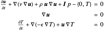
where ![]() is the temperature,
is the temperature, ![]() the diffusion coefficient and
the diffusion coefficient and ![]() the kinematic viscosity.
the kinematic viscosity.
Use the material parameters specified.
ClearAll[ν]
op = {
	u^(1, 0, 0)[t, x, y] + Inactive[Div][(-ν)*Inactive[Grad][u[t, x, y], {x, y}], {x, y}] + {u[t, x, y], v[t, x, y]}.Inactive[Grad][u[t, x, y], {x, y}] + p^(0, 1, 0)[t, x, y],
	v^(1, 0, 0)[t, x, y] + Inactive[Div][(-ν)*Inactive[Grad][v[t, x, y], {x, y}], {x, y}] + {u[t, x, y], v[t, x, y]}.Inactive[Grad][v[t, x, y], {x, y}] + p^(0, 0, 1)[t, x, y] - T[t, x, y],
	u^(0, 1, 0)[t, x, y] + v^(0, 0, 1)[t, x, y],
	T^(1, 0, 0)[t, x, y] + Inactive[Div][(-ϵ)*Inactive[Grad][T[t, x, y], {x, y}], {x, y}] + {u[t, x, y], v[t, x, y]}.Inactive[Grad][T[t, x, y], {x, y}]} /. parameters;
Boundary conditions and initial conditions need to be set up.
Again, the component could have been generated with the functions FluidFlowPDEComponent and HeatTransferPDEComponent.
wall = DirichletCondition[{u[t, x, y] == 0, v[t, x, y] == 0}, True];reference = DirichletCondition[p[t, x, y] == 0, x == 0 && y == 0];temperatures = {DirichletCondition[T[t, x, y] == 1, x == 0], DirichletCondition[T[t, x, y] == 0, x == length]};bcs = {wall, reference, temperatures} /. sizes;ic = {u[0, x, y] == 0, v[0, x, y] == 0, p[0, x, y] == 0, T[0, x, y] == 0};Monitor the time integration progress and the total time it takes to solve the PDE while using a refined mesh and interpolating the velocities ![]() and
and ![]() and the temperature
and the temperature ![]() with second order and the pressure
with second order and the pressure ![]() with first order.
with first order.
Monitor[AbsoluteTiming[
	{xVel, yVel, pressure, temperature} = NDSolveValue[{op == {0, 0, 0, 0}, bcs, ic}, {u, v, p, T}, {x, y}∈Ω, {t, 0, 300},
	Method -> {
	"PDEDiscretization" -> {"MethodOfLines",
	"SpatialDiscretization" -> {"FiniteElement", "MeshOptions" -> {"MaxCellMeasure" -> 0.00125}, "InterpolationOrder" -> {u -> 2, v -> 2, p -> 1, T -> 2}}}}
	, EvaluationMonitor :> (currentTime = Row[{"t = ", CForm[t]}])];
	], currentTime]
The last step is post-processing.
bmesh = ToBoundaryMesh[xVel["ElementMesh"]];
bmesh["Wireframe"]Show[ContourPlot[pressure[150, x, y], {x, y}∈pressure["ElementMesh"], ...], bmesh["Wireframe"]]Show[ContourPlot[temperature[150, x, y], {x, y}∈temperature["ElementMesh"], ...], bmesh["Wireframe"]]Show[bmesh["Wireframe"], VectorPlot[{xVel[150, x, y], yVel[150, x, y]}, {x, y}∈xVel["ElementMesh"], AspectRatio -> Automatic, PlotRange -> All]]numberOfFrames = 3;
frames = Table[Show[
bmesh["Wireframe"],
ContourPlot[temperature[t, x, y], {x, y}∈temperature["ElementMesh"], ...],
StreamPlot[{xVel[t, x, y], yVel[t, x, y]}, {x, y}∈xVel["ElementMesh"], ...]
], {t, 0, 300, 300 / numberOfFrames}];ListAnimate[frames, SaveDefinitions -> True]For the curious, investigate the different velocity field produced by simply swapping the cut-out positions.
RegionPlot[RegionDifference[RegionDifference[Rectangle[{0, 0}, {length, height}], Rectangle[{length / 2 + offset, height / 3}, {length / 2 + offset + thickness, height}]], Rectangle[{length / 2 - offset - thickness, 0}, {length / 2 - offset, 1 - height / 3}]] /. sizes, AspectRatio -> Automatic]More information about fluid flow, the Boussinesq approximation and applicable boundary conditions can be found in the Laminar Flow monograph and the Fluid Flow models guide page.