

LQEstimatorGains
LQEstimatorGains[ssm,{w,v}]
gives the optimal estimator gain matrix for the StateSpaceModel ssm, with process and measurement noise covariance matrices w and v.
LQEstimatorGains[ssm,{w,v,h}]
includes the cross-covariance matrix h.
LQEstimatorGains[{ssm,sensors},{…}]
specifies sensors as the noisy measurements of ssm.
LQEstimatorGains[{ssm,sensors,dinputs},{…}]
specifies dinputs as the deterministic inputs of ssm.
Details and Options
- The standard state-space model ssm can be given as StateSpaceModel[{a,b,c,d}] in either continuous time or discrete time:
-

continuous-time system 
discrete-time system - The descriptor state-space model ssm can be given as StateSpaceModel[{a,b,c,d,e}] in either continuous time or discrete time:
-

continuous-time system 
discrete-time system - LQEstimatorGains also accepts nonlinear systems specified by AffineStateSpaceModel and NonlinearStateSpaceModel.
- For nonlinear systems, the operating values of state and input variables are taken into consideration, and the gains are computed based on the approximate Taylor linearization.
- The input
 can include the process noise
  , as well as deterministic inputs
  .
. - The argument dinputs is a list of integers specifying the positions of
 in
in  .
. - The output
 consists of the noisy measurements
  as well as other outputs.
 - The argument sensors is a list of integers specifying the positions of
 in
in  .
. - LQEstimatorGains[ssm,{…}] is equivalent to LQEstimatorGains[{ssm,All,None},{…}].
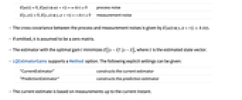
- The noisy measurements are modeled as
 , where
  and
and  are the submatrices of
  and
and  associated with
  , and
, and  is the noise.
 - The process and measurement noises are assumed to be white and Gaussian:
-
 ,
, 
process noise  ,
, 
measurement noise - The cross-covariance between the process and measurement noises is given by
 .
. - If omitted, h is assumed to be a zero matrix.
- The estimator with the optimal gain
 minimizes
  , where
  is the estimated state vector.
 - LQEstimatorGains supports a Method option. The following explicit settings can be given:
-
"CurrentEstimator" constructs the current estimator "PredictionEstimator" constructs the prediction estimator - The current estimate is based on measurements up to the current instant.
- The prediction estimate is based on measurements up to the previous instant.
- For continuous-time systems, the current and prediction estimators are the same. The optimal gain is computed as
 , where
  is the solution of the continuous algebraic Riccati equation
  . The matrix
  is the submatrix of
  associated with the process noise.
 - For discrete-time systems, the optimal gain
 of the current estimator is computed as
  , where
  is the solution of the discrete Riccati equation
  .
. - The optimal gain
 of the prediction estimator for a discrete-time system is computed as
  .
. - The optimal estimator is asymptotically stable if
 is nonsingular, the pair
  is detectable, and
  is stabilizable for any
  .
.
Examples
open all close allBasic Examples (3)
Scope (7)
Determine the optimal estimator gains of a continuous-time system:
The gains for a discrete-time system with nonzero cross-covariance:
The Kalman gains for a continuous-time system with cross-correlated noises:
Use the first output as the measurement:
Use the second output as the measurement:
The Kalman gains for a system in which the last four inputs are stochastic disturbances:
Estimator gain for a system with two deterministic inputs and two stochastic inputs:
The poles of the Kalman estimator:
Find the optimal gains for a descriptor state-space model:
The gains for an AffineStateSpaceModel:
Applications (1)
Properties & Relations (4)
Compute the Kalman estimator gains using the underlying Riccati equation:
LQEstimatorGains gives the same result:
The gains for a discrete-time system can be computed using DiscreteRiccatiSolve:
LQEstimatorGains gives the same result:
It is equivalent to the conjugate transpose of optimal regulator gains of the dual system:
Text
Wolfram Research (2010), LQEstimatorGains, Wolfram Language function, https://reference.wolfram.com/language/ref/LQEstimatorGains.html (updated 2014).
CMS
Wolfram Language. 2010. "LQEstimatorGains." Wolfram Language & System Documentation Center. Wolfram Research. Last Modified 2014. https://reference.wolfram.com/language/ref/LQEstimatorGains.html.
APA
Wolfram Language. (2010). LQEstimatorGains. Wolfram Language & System Documentation Center. Retrieved from https://reference.wolfram.com/language/ref/LQEstimatorGains.html