

SystemModelSimulate
SystemModelSimulate[model]
simulates model according to experiment settings.
SystemModelSimulate[model,tmax]
simulates from 0 to tmax.
SystemModelSimulate[model,{tmin,tmax}]
simulates from tmin to tmax.
SystemModelSimulate[model,vars,{tmin,tmax}]
stores only simulation data for the variables vars.
Details and Options
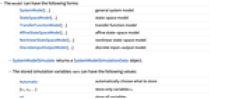
- The model can have the following forms:
-
SystemModel[…] general system model StateSpaceModel[…] state-space model TransferFunctionModel[…] transfer function model AffineStateSpaceModel[…] affine state-space model NonlinearStateSpaceModel[…] nonlinear state-space model DiscreteInputOutputModel[…] discrete input-output model - SystemModelSimulate returns a SystemModelSimulationData object.
- The stored simulation variables vars can have the following values:
-
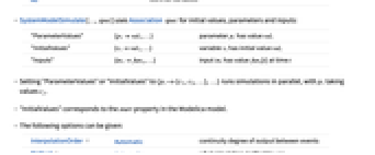
Automatic automatically choose what to store {v1,v2,…} store only variables vi All store all variables - SystemModelSimulate[…,spec] uses Association spec for initial values, parameters and inputs:
-
"ParameterValues" {p1val1,…} parameter pi has value vali "InitialValues" {v1val1,…} variable vi has initial value vali "Inputs" {in1fun1,…} input ini has value funi[t] at time t - Setting "ParameterValues" or "InitialValues" to {pi->{c1,c2,…},…} runs simulations in parallel, with pi taking values cj.
- "InitialValues" corresponds to the start property in the Modelica model.
- The following options can be given:
-
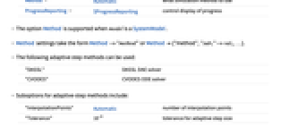
InterpolationOrder Automatic continuity degree of output between events Method Automatic what simulation method to use ProgressReporting $ProgressReporting control display of progress - The option Method is supported when model is a SystemModel.
- Method settings take the form Method->"method" or Method{"method","sub1"->val1,…}.
- The following adaptive step methods can be used:
-
"DASSL" DASSL DAE solver "CVODES" CVODES ODE solver - Suboptions for adaptive-step methods include:
-
"InterpolationPoints" Automatic number of interpolation points "Tolerance" 10-6 tolerance for adaptive step size - The following fixed-step methods can be used:
-
"Euler" explicit Euler's method of order 1 "Heun" Heun's method of order 2 "RungeKutta" explicit Runge–Kutta method of order 4 - Suboptions for fixed-step methods include:
-
"StepSize" 10-3 fixed step size - With Method->{"NDSolve",sub1->val1,…}, NDSolve is used as the solver. Method options subi are passed to NDSolve.
Examples
open all close allBasic Examples (3)
Scope (22)
Models (5)
Simulate one of the included example models from the thermal domain:
Simulate a NonlinearStateSpaceModel and plot simulation results:
Simulate a TransferFunctionModel with a UnitStep as input:
Do a parameter sweep in an AffineStateSpaceModel:
Simulate a DiscreteInputOutputModel:
Simulation Time (4)
Simulate with settings from the model:
Simulate for an explicit time interval:
Use a Quantity to specify the time interval:
Variables, Parameters and Inputs (8)
Initial values for variables can be set using "InitialValues":
Parameter values can be set using "ParameterValues":
Simulate a model that adds two inputs together:
Plot the inputs and the output:
Simulate for different initial values for the variable x:
Plot the variable x from all simulations:
Simulate a model with default parameters:
Set a parameter in the simulation:
Compare the variable ![]() between the simulations:
between the simulations:
Do a parameter sweep over a voltage offset:
Plot the voltage for all simulations:
Setting ranges for two parameters simulates once for each position in the ranges:
Simulate a model with a TimeSeries as input:
Simulation Results (5)
Simulate a model and plot the variables x1 and x2:
Get simulation results for the variables x and x':
Plot the variables using the Plot function:
Simulate a model and find the maximum of a variable:
Get the value of the variable angle1v:
Find the maximum value of the angle:
Run a simulation and plot in a single call:
Specify arguments to SystemModelSimulate:
Generalizations & Extensions (1)
Options (10)
InterpolationOrder (1)
Method (8)
Show the result in a ParametricPlot:
For stiff problems, use an adaptive-step method:
Simulating with too few interpolation points can give inexact plots:
Increasing the number of points gives a better result:
The default step size for a fixed-step solver might be smaller than needed:
Use a larger step size to speed up computation:
Let an adaptive solver choose the solver steps:
Use NDSolve for simulating a model:
The result is a SystemModelSimulationData object containing the simulation results:
Pass options to NDSolve:
ProgressReporting (1)
Control progress reporting with ProgressReporting:
Applications (11)
Calculate the overshoot of the height in a tank system:
Get the value of the step sent in to the tank:
Calculate the rise time for the height in a tank system:
Get the required values at 10% and 90% by looking at the steady-state value for height:
Find the times at which the signal reaches these values:
Plot lines at the final value, and when the signal reaches 10% and 90% of the final value:
Calculate the settling time for the height in a tank system:
Find 5% bounds on the final value:
Find the time at which the signal stays within these values:
Plot the bounds and the found settling time:
Change parameter values interactively:
Simulate a rolling wheel for different starting inertias along the wheel axis:
Fetch the trajectories for the wheel:
Analyze resonance peaks when varying a spring constant:
Calibrate parameters in a model by comparing to measurement data:
Set up a criteria function for model fitting:
Fit parameters to the test data:
Simulate with the fitted parameters:
Show the test data and the calibrated model together:
Filter sampled data from a Tinker Forge Weather Station:
Time shift and retrieve the magnitude of the data:
Run the time series through a lowpass filter:
Simulate a lowpass filter with sound as input:
Simulate with given input sound:
Retrieve the audio for input and output:
Fetch trajectories from the result:
Visualize simulated data with a WaveletScalogram:
Pick out the data you are interested in:
Properties & Relations (3)
The output from SystemModelSimulate is a SystemModelSimulationData object:
Use properties to get variable trajectories:
Use SystemModelSimulateSensitivity to also get sensitivities to parameters:
Plot the capacitor's voltage sensitivity to the frequency of "sineVoltage1":
Use SystemModelParametricSimulate for a function that can be evaluated for different values:
Compute solutions for different values of the frequency parameter:
Related Links
Text
Wolfram Research (2018), SystemModelSimulate, Wolfram Language function, https://reference.wolfram.com/language/ref/SystemModelSimulate.html (updated 2022).
CMS
Wolfram Language. 2018. "SystemModelSimulate." Wolfram Language & System Documentation Center. Wolfram Research. Last Modified 2022. https://reference.wolfram.com/language/ref/SystemModelSimulate.html.
APA
Wolfram Language. (2018). SystemModelSimulate. Wolfram Language & System Documentation Center. Retrieved from https://reference.wolfram.com/language/ref/SystemModelSimulate.html