Calculus
Calculus
| D[f,x] | partial derivative |
| D[f,x,y,…] | multiple derivative |
| D[f,{x,n}] | n th derivative |
| D[f,x,NonConstants->{v1,v2,…}] |
D[x ^ n, x]D[x ^ n, {x, 3}]You can differentiate with respect to any expression that does not involve explicit mathematical operations:
D[x[1] ^ 2 + x[2] ^ 2, x[1]]D[x ^ 2 + y ^ 2, x]If y does in fact depend on x, you can use the explicit functional form y[x]. "The Representation of Derivatives" describes how objects like y'[x] work:
D[x ^ 2 + y[x] ^ 2, x]Instead of giving an explicit function y[x], you can tell D that y implicitly depends on x. D[y,x,NonConstants->{y}] then represents  , with y implicitly depending on x:
D[x ^ 2 + y ^ 2, x, NonConstants -> {y}]| D[f,{{x1,x2,…}}] | the gradient of a scalar function |
| D[f,{{x1,x2,…},2}] | the Hessian matrix for f |
| D[f,{{x1,x2,…},n}] | the n th-order Taylor series coefficient |
| D[{f1,f2,…},{{x1,x2,…}}] | the Jacobian for a vector function f |
D[x ^ 2 + y ^ 2, {{x, y}}]D[x ^ 2 + y ^ 2, {{x, y}, 2}]D[{x ^ 2 + y ^ 2, x y}, {{x, y}}]| Dt[f] | total differential df |
| Dt[f,x] | total derivative |
| Dt[f,x,y,…] | multiple total derivative |
| Dt[f,x,Constants->{c1,c2,…}] | total derivative with ci constant (i.e. dci=0) |
| y/:Dt[y,x]=0 | set |
| SetAttributes[c,Constant] | define c to be a constant in all cases |
When you find the derivative of some expression  with respect to
  , you are effectively finding out how fast
  changes as you vary
  . Often
  will depend not only on
  , but also on other variables, say
  and
and  . The results that you get then depend on how you assume that
  and
and  vary as you change
  .
.
There are two common cases. Either  and
and  are assumed to stay fixed when
  changes, or they are allowed to vary with
  . In a standard partial derivative
  , all variables other than
  are assumed fixed. On the other hand, in the total derivative
  , all variables are allowed to change with
  .
.
In the Wolfram System, D[f,x] gives a partial derivative, with all other variables assumed independent of x. Dt[f,x] gives a total derivative, in which all variables are assumed to depend on x. In both cases, you can add an argument to give more information on dependencies.
D[x ^ 2 + y ^ 2, x]Dt[x ^ 2 + y ^ 2, x]% /. Dt[y, x] -> ypYou can also make an explicit definition for  . You need to use y/: to make sure that the definition is associated with y:
y/:Dt[y, x] = 0Dt[x ^ 2 + y ^ 2 + z ^ 2, x]Clear[y]Dt[x ^ 2 + y ^ 2 + z ^ 2, x, Constants -> {z}]SetAttributes[c, Constant]Dt[a ^ 2 + c x ^ 2, x]Dt[a ^ 2 + c[x] x ^ 2, x]Dt[x ^ 2 + c y ^ 2]% /. Dt[y] -> dyD[Log[x] ^ 2, x]D[f[x] ^ 2, x]The Wolfram Language applies the chain rule for differentiation, and leaves the result in terms of f':
D[x f[x ^ 2], x]D[%, x]When a function has more than one argument, superscripts are used to indicate how many times each argument is being differentiated:
D[g[x ^ 2, y ^ 2], x]This represents  . The Wolfram Language assumes that the order in which derivatives are taken with respect to different variables is irrelevant:
D[g[x, y], x, x, y]% /. x -> 0| f '[x] | first derivative of a function of one variable |
| f(n)[x] | n th derivative of a function of one variable |
| f(n1,n2,… )[x] | derivative of a function of several variables, ni times with respect to variable i |
Derivatives in the Wolfram System work essentially the same as in standard mathematics. The usual mathematical notation, however, often hides many details. To understand how derivatives are represented in the Wolfram System, you must look at these details.
The standard mathematical notation  is really a shorthand for
  , where
  is a "dummy variable". Similarly,
  is a shorthand for
  . As suggested by the notation
  , the object
  can in fact be viewed as a "pure function", to be evaluated with a particular choice of its parameter
  . You can think of the operation of differentiation as acting on a function
  , to give a new function, usually called
  .
.
With functions of more than one argument, the simple notation based on primes breaks down. You cannot tell, for example, whether  stands for
  or
or  , and for almost any
  , these will have totally different values. Once again, however,
  is just a dummy variable, whose sole purpose is to show with respect to which "slot"
  is to be differentiated.
In the Wolfram System, as in some branches of mathematics, it is convenient to think about a kind of differentiation that acts on functions, rather than expressions. An operation is needed that takes the function  , and gives the derivative function
  . Operations such as this that act on functions, rather than variables, are known in mathematics as operators.
The object f' in the Wolfram System is the result of applying the differentiation operator to the function f. The full form of f' is in fact Derivative[1][f]. Derivative[1] is the Wolfram System differentiation operator.
The arguments in the operator Derivative[n1,n2,…] specify how many times to differentiate with respect to each "slot" of the function on which it acts. By using operators to represent differentiation, the Wolfram System avoids any need to introduce explicit "dummy variables".
f'//FullFormf'[x]//FullFormf''[x]//FullFormD[g[x, y], y]%//FullFormHere is the second derivative with respect to the variable y, which appears in the second slot of g:
D[g[x, y], {y, 2}]//FullFormD[g[x, y], x, y, y]//FullFormSince Derivative only specifies how many times to differentiate with respect to each slot, the order of the derivatives is irrelevant:
D[g[x, y], y, y, x]//FullFormHere is a more complicated case, in which both arguments of g depend on the differentiation variable:
D[g[x, x], x]%//FullFormThe object f' behaves essentially like any other function in the Wolfram System. You can evaluate the function with any argument, and you can use standard the Wolfram System /. operations to change the argument. (This would not be possible if explicit dummy variables had been introduced in the course of the differentiation.)
This is the Wolfram System representation of the derivative of a function f, evaluated at the origin:
f'[0]//FullFormD[f[x ^ 2], x]You can evaluate the result at the point  by using the standard Wolfram System replacement operation:
% /. x -> 2There is some slight subtlety when you need to deduce the value of f' based on definitions for objects like f[x_].
h[x_] := x ^ 4When you take the derivative of h[x], the Wolfram System first evaluates h[x], then differentiates the result:
D[h[x], x]h'[x]h'The function f' is completely determined by the form of the function f. Definitions for objects like f[x_] do not immediately apply, however, to expressions like f'[x]. The problem is that f'[x] has the full form Derivative[1][f][x], which nowhere contains anything that explicitly matches the pattern f[x_]. In addition, for many purposes it is convenient to have a representation of the function f' itself, without necessarily applying it to any arguments.
What the Wolfram System does is to try and find the explicit form of a pure function which represents the object f'. When the Wolfram System gets an expression like Derivative[1][f], it effectively converts it to the explicit form D[f[#],#]& and then tries to evaluate the derivative. In the explicit form, the Wolfram System can immediately use values that have been defined for objects like f[x_]. If the Wolfram System succeeds in doing the derivative, it returns the explicit pure‐function result. If it does not succeed, it leaves the derivative in the original f' form.
Tan'%[y]You can define the derivative in the Wolfram Language of a function f of one argument simply by an assignment like f'[x_]=fp[x].
f'[x_] := fp[x]D[f[x ^ 2], x]D[%, x]g'[0] = g0D[g[x] ^ 2, x] /. x -> 0g''[x_] = gpp[x]D[g[x] ^ 2, {x, 2}]To define derivatives of functions with several arguments, you have to use the general representation of derivatives in the Wolfram Language.
| f'[x_]:=rhs | define the first derivative of f |
| Derivative[n][f][x_]:=rhs | define the n th derivative of f |
| Derivative[m,n,…][g][x_,_,…]:=rhs | |
define derivatives of g with respect to various arguments | |
Derivative[0, 2][g][x_, y_] := g2p[x, y]D[g[a ^ 2, x ^ 2], x, x]Integrate[x ^ n, x]Integrate[1 / (x ^ 4 - a ^ 4), x]The Wolfram Language knows how to do almost any integral that can be done in terms of standard mathematical functions. But you should realize that even though an integrand may contain only fairly simple functions, its integral may involve much more complicated functions—or may not be expressible at all in terms of standard mathematical functions.
Integrate[Log[1 - x ^ 2], x]Integrate[Log[1 - x ^ 2] / x, x]This integral involves Erf:
Integrate[Exp[1 - x ^ 2], x]Integrate[Sin[x ^ 2], x]Integrate[(1 - x ^ 2) ^ n, x]This integral simply cannot be done in terms of standard mathematical functions. As a result, the Wolfram Language just leaves it undone:
Integrate[x ^ x, x]| Integrate[f,x] | the indefinite integral ∫f dx |
| Integrate[f,x,y] | the multiple integral ∫dx dy f |
| Integrate[f,{x,xmin,xmax}] | the definite integral |
| Integrate[f,{x,xmin,xmax},{y,ymin,ymax}] | |
the multiple integral | |
Integrate[Sin[x] ^ 2, {x, a, b}]Integrate[Exp[-x ^ 2], {x, 0, Infinity}]Integrate[x ^ x, {x, 0, 1}]N[%]This evaluates the multiple integral  . The range of the outermost integration variable appears first:
Integrate[x ^ 2 + y ^ 2, {x, 0, 1}, {y, 0, x}]Integrate[x ^ 10 Boole[x ^ 2 + y ^ 2 <= 1], {x, -1, 1}, {y, -1, 1}]The Wolfram Language function Integrate[f,x] gives you the indefinite integral  . You can think of the operation of indefinite integration as being an inverse of differentiation. If you take the result from Integrate[f,x], and then differentiate it, you always get a result that is mathematically equal to the original expression f.
In general, however, there is a whole family of results which have the property that their derivative is f. Integrate[f,x] gives you an expression whose derivative is f. You can get other expressions by adding an arbitrary constant of integration, or indeed by adding any function that is constant except at discrete points.
If you fill in explicit limits for your integral, any such constants of integration must cancel out. But even though the indefinite integral can have arbitrary constants added, it is still often very convenient to manipulate it without filling in the limits.
Integrate[x ^ 2, x]You can add an arbitrary constant to the indefinite integral, and still get the same derivative. Integrate simply gives you an expression with the required derivative:
D[% + c, x]Integrate[1 / (x ^ 2 - 1), x]D[%, x]Simplify[%]The Integrate function assumes that any object that does not explicitly contain the integration variable is independent of it, and can be treated as a constant. As a result, Integrate is like an inverse of the partial differentiation function D.
Integrate[a x ^ 2, x]The integration variable can be any expression that does not involve explicit mathematical operations:
Integrate[x b[x] ^ 2, b[x]]Another assumption that Integrate implicitly makes is that all the symbolic quantities in your integrand have "generic" values. Thus, for example, the Wolfram Language will tell you that  is
is  even though this is not true in the special case
  .
.
The Wolfram Language gives the standard result for this integral, implicitly assuming that n is not equal to -1:
Integrate[x ^ n, x]Integrate[x ^ -1, x]You should realize that the result for any particular integral can often be written in many different forms. The Wolfram Language tries to give you the most convenient form, following principles such as avoiding explicit complex numbers unless your input already contains them.
This integral is given in terms of ArcTan:
Integrate[1 / (1 + a x ^ 2), x]This integral is given in terms of ArcTanh:
Integrate[1 / (1 - b x ^ 2), x]% /. b -> -aD[%, x]Even though they look quite different, both ArcTan[x] and -ArcTan[1/x] are indefinite integrals of  :
:
Simplify[D[{ArcTan[x], -ArcTan[1 / x]}, x]]Integrate chooses to use the simpler of the two forms:
Integrate[1 / (1 + x ^ 2), x]Evaluating integrals is much more difficult than evaluating derivatives. For derivatives, there is a systematic procedure based on the chain rule that effectively allows any derivative to be worked out. But for integrals, there is no such systematic procedure.
One of the main problems is that it is difficult to know what kinds of functions will be needed to evaluate a particular integral. When you work out a derivative, you always end up with functions that are of the same kind or simpler than the ones you started with. But when you work out integrals, you often end up needing to use functions that are much more complicated than the ones you started with.
Integrate[Log[x] ^ 2, x]But for this integral the special function LogIntegral is needed:
Integrate[Log[Log[x]], x]Integrate[Sin[x ^ 2], x]This integral involves an incomplete gamma function. Note that the power is carefully set up to allow any complex value of x:
Integrate[Exp[-x ^ a], x]The Wolfram Language includes a very wide range of mathematical functions, and by using these functions a great many integrals can be done. But it is still possible to find even fairly simple‐looking integrals that just cannot be done in terms of any standard mathematical functions.
Here is a fairly simple‐looking integral that cannot be done in terms of any standard mathematical functions:
Integrate[Sin[x] / Log[x], x]The main point of being able to do an integral in terms of standard mathematical functions is that it lets one use the known properties of these functions to evaluate or manipulate the result one gets.
In the most convenient cases, integrals can be done purely in terms of elementary functions such as exponentials, logarithms and trigonometric functions. In fact, if you give an integrand that involves only such elementary functions, then one of the important capabilities of Integrate is that if the corresponding integral can be expressed in terms of elementary functions, then Integrate will essentially always succeed in finding it.
Integrals of rational functions are straightforward to evaluate, and always come out in terms of rational functions, logarithms and inverse trigonometric functions:
Integrate[x / ((x - 1)(x + 2)), x]The integral here is still of the same form, but now involves an implicit sum over the roots of a polynomial:
Integrate[1 / (1 + 2 x + x ^ 3), x]N[%]Integrate[Sin[x] ^ 3 Cos[x] ^ 2, x]Integrate[Sqrt[x] Sqrt[1 + x], x]Integrate[Sqrt[x + Sqrt[x]], x]By nesting elementary functions you sometimes get integrals that can be done in terms of elementary functions:
Integrate[Cos[Log[x]], x]Integrate[Log[Cos[x]], x]Integrate[Sqrt[Cos[x]], x]Integrate[Sqrt[Tan[x]], x]Integrals like this can systematically be done using Piecewise:
Integrate[2 ^ Max[x, 1 - x], x]Beyond working with elementary functions, Integrate includes a large number of algorithms for dealing with special functions. Sometimes it uses a direct generalization of the procedure for elementary functions. But more often its strategy is first to try to write the integrand in a form that can be integrated in terms of certain sophisticated special functions, and then having done this to try to find reductions of these sophisticated functions to more familiar functions.
Integrate[BesselJ[0, x], x]Integrate[x ^ 3 BesselJ[0, x], x]A large book of integral tables will list perhaps a few thousand indefinite integrals. The Wolfram Language can do essentially all of these integrals. And because it contains general algorithms rather than just specific cases, the Wolfram Language can actually do a vastly wider range of integrals.
Integrate[Log[1 - x] / x, x]To do this integral, however, requires a more general algorithm, rather than just a direct table lookup:
Integrate[Log[1 + 3 x + x ^ 2] / x, x]Particularly if you introduce new mathematical functions of your own, you may want to teach the Wolfram Language new kinds of integrals. You can do this by making appropriate definitions for Integrate.
In the case of differentiation, the chain rule allows one to reduce all derivatives to a standard form, represented in the Wolfram Language using Derivative. But for integration, no such similar standard form exists, and as a result you often have to make definitions for several different versions of the same integral. Changes of variables and other transformations can rarely be done automatically by Integrate.
This integral cannot be done in terms of any of the standard mathematical functions built into the Wolfram Language:
Integrate[Sin[Sin[x]], x]Unprotect[Integrate]Integrate[Sin[Sin[a_. + b_. x_]], x_] := Jones[a, x] / bIntegrate[Sin[Sin[3x]], x]As it turns out, the integral  can in principle be represented as an infinite sum of
  hypergeometric functions, or as a suitably generalized Kampé de Fériet hypergeometric function of two variables.
| Integrate[f,x] | the indefinite integral |
| Integrate[f,{x,xmin,xmax}] | the definite integral |
| Integrate[f,{x,xmin,xmax},{y,ymin,ymax}] | |
the multiple integral | |
Integrate[x ^ 2, {x, a, b}]Integrate[x ^ 2 + y ^ 2, {x, 0, a}, {y, 0, b}]The y integral is done first. Its limits can depend on the value of x. This ordering is the same as is used in functions like Sum and Table:
Integrate[x ^ 2 + y ^ 2, {x, 0, a}, {y, 0, x}]In simple cases, definite integrals can be done by finding indefinite forms and then computing appropriate limits. But there is a vast range of integrals for which the indefinite form cannot be expressed in terms of standard mathematical functions, but the definite form still can be.
Integrate[Cos[Sin[x]], x]Integrate[Cos[Sin[x]], {x, 0, 2Pi}]Here is an integral where the indefinite form can be found, but it is much more efficient to work out the definite form directly:
Integrate[Log[x] Exp[-x ^ 2], {x, 0, Infinity}]Just because an integrand may contain special functions, it does not mean that the definite integral will necessarily be complicated:
Integrate[BesselK[0, x] ^ 2, {x, 0, Infinity}]Integrate[BesselK[0, x] BesselJ[0, x], {x, 0, Infinity}]Integrate[Sin[x ^ 2] Exp[-x], {x, 0, Infinity}]Even when you can find the indefinite form of an integral, you will often not get the correct answer for the definite integral if you just subtract the values of the limits at each end point. The problem is that within the domain of integration there may be singularities whose effects are ignored if you follow this procedure.
Integrate[1 / x ^ 2, x]Limit[%, x -> 2] - Limit[%, x -> -2]Integrate[1 / x ^ 2, {x, -2, 2}]Integrate[1 / (1 + a Sin[x]), x]Limit[%, x -> 2Pi] - Limit[%, x -> 0]The definite integral, however, gives the correct result which depends on  . The assumption assures convergence:
Integrate[1 / (1 + a Sin[x]), {x, 0, 2Pi}, Assumptions -> -1 < a < 1]| Integrate[f,{x,xmin,xmax},PrincipalValue->True] | |
the Cauchy principal value of a definite integral | |
Integrate[1 / x, x]Limit[%, x -> 2] - Limit[%, x -> -1]Integrate[1 / x, {x, -1, 2}]Integrate[1 / x, {x, -1, 2}, PrincipalValue -> True]When parameters appear in an indefinite integral, it is essentially always possible to get results that are correct for almost all values of these parameters. But for definite integrals this is no longer the case. The most common problem is that a definite integral may converge only when the parameters that appear in it satisfy certain specific conditions.
Integrate[x ^ n, x]For the definite integral, however,  must satisfy a condition in order for the integral to be convergent:
Integrate[x ^ n, {x, 0, 1}]% /. n -> 2option name | default value | |
| GenerateConditions | Automatic | whether to generate explicit conditions |
| Assumptions | $Assumptions | what relations about parameters to assume |
Options for Integrate.
Integrate[x ^ n, {x, 0, 1}, Assumptions -> (n > 2)]Even when a definite integral is convergent, the presence of singularities on the integration path can lead to discontinuous changes when the parameters vary. Sometimes a single formula containing functions like Sign can be used to summarize the result. In other cases, however, an explicit If is more convenient.
The If here gives the condition for the integral to be convergent:
Integrate[Sin[a x] / x, {x, 0, Infinity}]Integrate[Sin[a x] / x, {x, 0, Infinity}, Assumptions -> Im[a] == 0]The result is discontinuous as a function of  . The discontinuity can be traced to the essential singularity of
  at
at  :
:
Plot[%, {a, -5, 5}]There is no convenient way to represent this answer in terms of Sign, so the Wolfram Language generates an explicit If:
Integrate[Sin[x] BesselJ[0, a x] / x, {x, 0, Infinity}, Assumptions -> Im[a] == 0]Plot[Evaluate[%], {a, -5, 5}]Integrate[If[x ^ 2 + y ^ 2 < 1, 1, 0], {x, -1, 1}, {y, -1, 1}]Integrate[Boole[x ^ 2 + y ^ 2 < 1], {x, -1, 1}, {y, -1, 1}]Even though an integral may be straightforward over a simple rectangular region, it can be significantly more complicated even over a circular region.
Integrate[Exp[x] Boole[x ^ 2 + y ^ 2 < 1], {x, -1, 1}, {y, -1, 1}]Particularly if there are parameters inside the conditions that define regions, the results for integrals over regions may break into several cases.
Integrate[Boole[a x < y], {x, 0, 1}, {y, 0, 1}]Integrate[Boole[a x < b], {x, 0, 1}]Integrate[Boole[x ^ 2 + y ^ 2 < a], {x, 0, 1}, {y, 0, 1}]Integrate[Boole[Sin[x] > 1 / 2] Exp[-x], {x, 0, Infinity}]When the Wolfram Language cannot give you an explicit result for an integral, it leaves the integral in a symbolic form. It is often useful to manipulate this symbolic form.
The Wolfram Language cannot give an explicit result for this integral, so it leaves the integral in symbolic form:
Integrate[x ^ 2 f[x], x]D[%, x]Integrate[f[x], {x, a[x], b[x]}]D[%, x]defint = Integrate[f[x], {x, a, b}]D[defint, u]Dt[defint, u]You can use the Wolfram Language function DSolve to find symbolic solutions to ordinary and partial differential equations.
Solving a differential equation consists essentially in finding the form of an unknown function. In the Wolfram Language, unknown functions are represented by expressions like y[x]. The derivatives of such functions are represented by y'[x], y''[x], and so on.
The Wolfram Language function DSolve returns as its result a list of rules for functions. There is a question of how these functions are represented. If you ask DSolve to solve for y[x], then DSolve will indeed return a rule for y[x]. In some cases, this rule may be all you need. But this rule, on its own, does not give values for y'[x] or even y[0]. In many cases, therefore, it is better to ask DSolve to solve not for y[x], but instead for y itself. In this case, what DSolve will return is a rule which gives y as a pure function, in the sense discussed in "Pure Functions".
DSolve[y'[x] + y[x] == 1, y[x], x]y[x] + 2y'[x] + y[0] /. %DSolve[y'[x] + y[x] == 1, y, x]y[x] + 2y'[x] + y[0] /. %Substituting the solution into the original equation yields True:
y'[x] + y[x] == 1 /. %%| DSolve[eqn,y[x],x] | solve a differential equation for y[x] |
| DSolve[eqn,y,x] | solve a differential equation for the function y |
In standard mathematical notation, one typically represents solutions to differential equations by explicitly introducing "dummy variables" to represent the arguments of the functions that appear. If all you need is a symbolic form for the solution, then introducing such dummy variables may be convenient. However, if you actually intend to use the solution in a variety of other computations, then you will usually find it better to get the solution in pure‐function form, without dummy variables. Notice that this form, while easy to represent in the Wolfram Language, has no direct analog in standard mathematical notation.
| DSolve[{eqn1,eqn2,…},{y1,y2,…},x] | |
solve a list of differential equations | |
DSolve[{y[x] == -z'[x], z[x] == -y'[x]}, {y, z}, x]DSolve[y[x] y'[x] == 1, y, x]You can add constraints and boundary conditions for differential equations by explicitly giving additional equations such as y[0]==0.
DSolve[{y'[x] == a y[x], y[0] == 1}, y[x], x]If you ask the Wolfram Language to solve a set of differential equations and you do not give any constraints or boundary conditions, then the Wolfram Language will try to find a general solution to your equations. This general solution will involve various undetermined constants. One new constant is introduced for each order of derivative in each equation you give.
The default is that these constants are named C[n], where the index n starts at 1 for each invocation of DSolve. You can override this choice, by explicitly giving a setting for the option GeneratedParameters. Any function you give is applied to each successive index value n to get the constants to use for each invocation of DSolve.
DSolve[y''''[x] == y[x], y[x], x]Each independent initial or boundary condition you give reduces the number of undetermined constants by one:
DSolve[{y''''[x] == y[x], y[0] == y'[0] == 0}, y[x], x]You should realize that finding exact formulas for the solutions to differential equations is a difficult matter. In fact, there are only fairly few kinds of equations for which such formulas can be found, at least in terms of standard mathematical functions.
The most widely investigated differential equations are linear ones, in which the functions you are solving for, as well as their derivatives, appear only linearly.
DSolve[y'[x] - x y[x] == 0, y[x], x]DSolve[y'[x] - x y[x] == 1, y[x], x]If you have only a single linear differential equation, and it involves only a first derivative of the function you are solving for, then it turns out that the solution can always be found just by doing integrals.
But as soon as you have more than one differential equation, or more than a first‐order derivative, this is no longer true. However, some simple second‐order linear differential equations can nevertheless be solved using various special functions from "Special Functions". Indeed, historically many of these special functions were first introduced specifically in order to represent the solutions to such equations.
DSolve[y''[x] - x y[x] == 0, y[x], x]DSolve[y''[x] - Exp[x] y[x] == 0, y[x], x]DSolve[y''[x] + Cos[x] y[x] == 0, y, x]DSolve[y''[x] - Cot[x] ^ 2 y[x] == 0, y[x], x]DSolve[x ^ 2 y''[x] + y[x] == 0, y[x], x]Beyond second order, the kinds of functions needed to solve even fairly simple linear differential equations become extremely complicated. At third order, the generalized Meijer G function MeijerG can sometimes be used, but at fourth order and beyond absolutely no standard mathematical functions are typically adequate, except in very special cases.
Here is a third‐order linear differential equation which can be solved in terms of generalized hypergeometric functions:
DSolve[y'''[x] + x y[x] == 0, y[x], x]DSolve[y'''[x] + Exp[x] y[x] == 0, y[x], x]For nonlinear differential equations, only rather special cases can usually ever be solved in terms of standard mathematical functions. Nevertheless, DSolve includes fairly general procedures which allow it to handle almost all nonlinear differential equations whose solutions are found in standard reference books.
First‐order nonlinear differential equations in which  does not appear on its own are fairly easy to solve:
DSolve[y'[x] - y[x] ^ 2 == 0, y[x], x]DSolve[y'[x] - y[x] ^ 2 == x, y[x], x]//FullSimplifyDSolve[y'[x] - x y[x] ^ 2 - y[x] == 0, y[x], x]DSolve[y'[x] - x y[x] ^ 3 + y[x] == 0, y[x], x]DSolve[y'[x] + x y[x] ^ 3 + y[x] ^ 2 == 0, y[x], x]In practical applications, it is quite often convenient to set up differential equations that involve piecewise functions. You can use DSolve to find symbolic solutions to such equations.
DSolve[y'[x] - y[x] == UnitStep[x], y[x], x]DSolve[y'[x] + Clip[x] y[x] == 0, y[x], x]Beyond ordinary differential equations, one can consider differential-algebraic equations that involve a mixture of differential and algebraic equations.
DSolve[{y'[x] + 3z'[x] == 4 y[x] + 1 / x, y[x] + z[x] == 1}, {y[x], z[x]}, x]| DSolve[eqn,y[x1,x2,…],{x1,x2,…}] | |
solve a partial differential equation for y[x1,x2,…] | |
| DSolve[eqn,y,{x1,x2,…}] | solve a partial differential equation for the function y |
DSolve is set up to handle not only ordinary differential equations in which just a single independent variable appears, but also partial differential equations in which two or more independent variables appear.
This finds the general solution to a simple partial differential equation with two independent variables:
DSolve[D[y[x1, x2], x1] + D[y[x1, x2], x2] == 1 / (x1 x2), y[x1, x2], {x1, x2}]DSolve[D[y[x1, x2], x1] + D[y[x1, x2], x2] == 1 / (x1 x2), y, {x1, x2}]The basic mathematics of partial differential equations is considerably more complicated than that of ordinary differential equations. One feature is that whereas the general solution to an ordinary differential equation involves only arbitrary constants, the general solution to a partial differential equation, if it can be found at all, must involve arbitrary functions. Indeed, with  independent variables, arbitrary functions of
  arguments appear. DSolve by default names these functions C[n].
(D[#, x1] + D[#, x2] + D[#, x3])&[y[x1, x2, x3]] == 0DSolve[%, y[x1, x2, x3], {x1, x2, x3}](c ^ 2 D[#, x, x] - D[#, t, t])&[y[x, t]] == 0DSolve[%, y[x, t], {x, t}]For an ordinary differential equation, it is guaranteed that a general solution must exist, with the property that adding initial or boundary conditions simply corresponds to forcing specific choices for arbitrary constants in the solution. But for partial differential equations this is no longer true. Indeed, it is only for linear partial differential and a few other special types that such general solutions exist.
Other partial differential equations can be solved only when specific initial or boundary values are given, and in the vast majority of cases no solutions can be found as exact formulas in terms of standard mathematical functions.
DSolve[x1 D[y[x1, x2], x1] + x2 D[y[x1, x2], x2] == Exp[x1 x2], y[x1, x2], {x1, x2}]DSolve[D[y[x1, x2], x1] + D[y[x1, x2], x2] == Exp[y[x1, x2]], y[x1, x2], {x1, x2}]//QuietDSolve[D[y[x1, x2], x1] D[y[x1, x2], x2] == a, y[x1, x2], {x1, x2}]Laplace Transforms
| LaplaceTransform[expr,t,s] | the Laplace transform of expr |
| InverseLaplaceTransform[expr,s,t] | the inverse Laplace transform of expr |
The Laplace transform of a function  is given by
 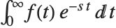 . The inverse Laplace transform of
  is given for suitable
  by
by 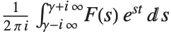 .
.
LaplaceTransform[t ^ 4 Sin[t], t, s]InverseLaplaceTransform[%, s, t]LaplaceTransform[1 / (1 + t ^ 2), t, s]LaplaceTransform[1 / (1 + t ^ 3), t, s]InverseLaplaceTransform returns the original function:
InverseLaplaceTransform[%, s, t]LaplaceTransform[BesselJ[n, t], t, s]Laplace transforms have the property that they turn integration and differentiation into essentially algebraic operations. They are therefore commonly used in studying systems governed by differential equations.
LaplaceTransform[Integrate[f[u], {u, 0, t}], t, s]| LaplaceTransform[expr,{t1,t2,…},{s1,s2,…}] | |
the multidimensional Laplace transform of expr | |
| InverseLaplaceTransform[expr,{s1,s2,…},{t1,t2,…}] | |
the multidimensional inverse Laplace transform of expr | |
Fourier Transforms
| FourierTransform[expr,t,ω] | the Fourier transform of expr |
| InverseFourierTransform[expr,ω,t] | the inverse Fourier transform of expr |
Integral transforms can produce results that involve "generalized functions" such as HeavisideTheta:
FourierTransform[1 / (1 + t ^ 4), t, ω]InverseFourierTransform[%, ω, t]In the Wolfram Language the Fourier transform of a function  is by default defined to be
 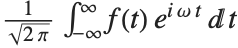 . The inverse Fourier transform of
  is similarly defined as
 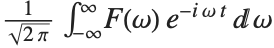 .
.
In different scientific and technical fields different conventions are often used for defining Fourier transforms. The option FourierParameters in the Wolfram Language allows you to choose any of these conventions you want.
common convention
|
setting
|
Fourier transform
|
inverse Fourier transform
|
Wolfram Language default |
{0,1}
| ||
pure mathematics |
{1,-1}
| ||
classical physics |
{-1,1}
| ||
modern physics |
{0,1}
| ||
systems engineering |
{1,-1}
| ||
signal processing |
{0,-2Pi}
| ||
general case |
{a,b}
|
Typical settings for FourierParameters with various conventions.
FourierTransform[Exp[-t ^ 2], t, ω]Here is the same Fourier transform with the choice of parameters typically used in signal processing:
FourierTransform[Exp[-t ^ 2], t, ω, FourierParameters -> {0, -2 Pi}]| FourierSinTransform[expr,t,ω] | Fourier sine transform |
| FourierCosTransform[expr,t,ω] | Fourier cosine transform |
| InverseFourierSinTransform[expr,ω,t] | |
inverse Fourier sine transform | |
| InverseFourierCosTransform[expr,ω,t] | |
inverse Fourier cosine transform | |
In some applications of Fourier transforms, it is convenient to avoid ever introducing complex exponentials. Fourier sine and cosine transforms correspond to integrating respectively with  and
and  instead of
  , and using limits 0 and
  rather than
  and
and  .
.
{FourierSinTransform[Exp[-t], t, ω], FourierCosTransform[Exp[-t], t, ω]}| FourierTransform[expr,{t1,t2,…},{ω1,ω2,…}] | |
the multidimensional Fourier transform of expr | |
| InverseFourierTransform[expr,{ω1,ω2,…},{t1,t2,…}] | |
the multidimensional inverse Fourier transform of expr | |
| FourierSinTransform[expr,{t1,t2,…},{ω1,ω2,…}]
,
FourierCosTransform[expr,{t1,t2,…},{ω1,ω2,…}] | |
the multidimensional sine and cosine Fourier transforms of expr | |
| InverseFourierSinTransform[expr,{ω1,ω2,…},{t1,t2,…}]
,
InverseFourierCosTransform[expr,{ω1,ω2,…},{t1,t2,…}] | |
the multidimensional inverse Fourier sine and cosine transforms of expr | |
FourierTransform[(u v) ^ 2 Exp[-u ^ 2 - v ^ 2], {u, v}, {a, b}]InverseFourierTransform[%, {a, b}, {u, v}]Z Transforms
| ZTransform[expr,n,z] | Z transform of expr |
| InverseZTransform[expr,z,n] | inverse Z transform of expr |
The Z transform of a function  is given by
  . The inverse Z transform of
  is given by the contour integral
  . Z transforms are effectively discrete analogs of Laplace transforms. They are widely used for solving difference equations, especially in digital signal processing and control theory. They can be thought of as producing generating functions, of the kind commonly used in combinatorics and number theory.
ZTransform[2 ^ -n, n, z]InverseZTransform[%, z, n]ZTransform[1 / n!, n, z]In many practical situations it is convenient to consider limits in which a fixed amount of something is concentrated into an infinitesimal region. Ordinary mathematical functions of the kind normally encountered in calculus cannot readily represent such limits. However, it is possible to introduce generalized functions or distributions which can represent these limits in integrals and other types of calculations.
| DiracDelta[x] | Dirac delta function |
| HeavisideTheta[x] | Heaviside theta function |
Plot[Sqrt[50 / Pi] Exp[-50 x ^ 2], {x, -2, 2}, PlotRange -> All]Plot[Evaluate[Sqrt[n / Pi] Exp[-n x ^ 2] /. n -> {1, 10, 100}], {x, -2, 2}, PlotRange -> All]Integrate[Sqrt[n / Pi] Exp[-n x ^ 2], {x, -Infinity, Infinity}, Assumptions -> n > 0]The limit of the functions for infinite  is effectively a Dirac delta function, whose integral is again 1:
Integrate[DiracDelta[x], {x, -Infinity, Infinity}]Table[DiracDelta[x], {x, -3, 3}]Inserting a delta function in an integral effectively causes the integrand to be sampled at discrete points where the argument of the delta function vanishes.
Integrate[DiracDelta[x - 2] f[x], {x, -4, 4}]Integrate[DiracDelta[x ^ 2 - x - 1], {x, 0, 2}]Integrate[DiracDelta[Cos[x]], {x, -30, 30}]The Heaviside function HeavisideTheta[x] is the indefinite integral of the delta function. It is variously denoted  ,
,  ,
,  , and
, and  . As a generalized function, the Heaviside function is defined only inside an integral. This distinguishes it from the unit step function UnitStep[x], which is a piecewise function.
Integrate[DiracDelta[x], x]Integrate[f[x] DiracDelta[x - a], {x, -2, 2}, Assumptions -> a ∈ Reals]FourierTransform[1, t, ω]FourierTransform[Cos[t], t, ω]Dirac delta functions can be used in DSolve to find the impulse response or Green's function of systems represented by linear and certain other differential equations.
DSolve[{x''[t] + r x[t] == DiracDelta[t], x[0] == 0, x'[0] == 1}, x[t], t] /. {HeavisideTheta[0] -> 1}| DiracDelta[x1,x2,…] | multidimensional Dirac delta function |
| HeavisideTheta[x1,x2,…] | multidimensional Heaviside theta function |
Multidimensional generalized functions are essentially products of univariate generalized functions.
D[HeavisideTheta[x, y, z], x]Related to the multidimensional Dirac delta function are two integer functions: discrete delta and Kronecker delta. Discrete delta  is 1 if all the
  , and is zero otherwise. Kronecker delta
  is 1 if all the
  are equal, and is zero otherwise.
| DiscreteDelta[n1,n2,…] | discrete delta |
| KroneckerDelta[n1,n2,…] | Kronecker delta |