|
2.9.7 AC Analysis of the CMOS Amplifier
To conclude this chapter let's carry out an AC analysis of the CMOS amplifier. Our task shall be to determine a symbolic formula which approximates the frequency response of the voltage gain to first order. We begin with importing the numerical data from the PSpice small-signal simulation applying the Analog Insydes command ReadSimulationData. Note that we have to specify the simulator-specific option setting Simulator -> "PSpice".
In[34]:= data = ReadSimulationData[
"AnalogInsydes/DemoFiles/CMOSdiffamp.csd",
Simulator -> "PSpice"]
Out[40]= 
In[35]:= tfcmosPSpice := "V(5)" /. First[data]
The Bode diagram of the simulation result shows that the transfer function has a dominant pole which is responsible for the corner in the magnitude response at  . .
In[36]:= BodePlot[tfcmosPSpice[f], {f, 1., 1.*10^9}]
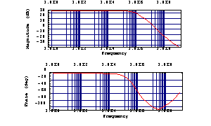
Out[42]= 
Next, we set up a system of circuit equations in symbolic form. Remember that this requires specifying the option ElementValues -> Symbolic in the call to CircuitEquations. Furthermore, we use a complexity-reduced device model for the transistors by the option setting ModelLibrary -> "BasicModels`" (see Section 3.14.4) as we shall not be interested in high-frequency parasitic effects.
In[37]:= stacmoshf = CircuitEquations[cmosdiffamp,
ElementValues -> Symbolic, Formulation -> SparseTableau,
ModelLibrary -> "BasicModels`"]
Out[43]= 
We can now perform a numerical reference simulation within Analog Insydes to ensure that the imported data is correct and that the employed transistor models are sufficient for computing the small-signal voltage gain and the subsequent symbolic approximations. The corresponding Analog Insydes command for carrying out a numerical small-signal analysis is ACAnalysis.
In[38]:= reference = ACAnalysis[stacmoshf, {V$CL}, {f, 1., 1.*^9}]
Out[44]= 
Within the Bode diagram we compare the results of the PSpice simulation and the Analog Insydes simulation. One can see that the curves match perfectly in the computed frequency range.
In[39]:= BodePlot[reference, {tfcmosPSpice[f], V$CL[f]},
{f, 1., 1.*10^9}, ShowLegend -> False]
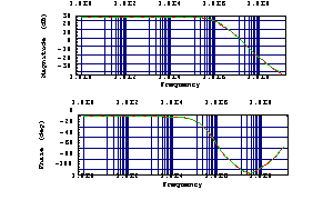
Out[45]= 
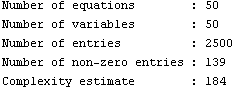
Following, we can proceed with carrying out the symbolic approximation. Note that statistical information concerning DAEObjects can be displayed via the Analog Insydes command Statistics:
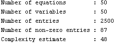
In[40]:= Statistics[stacmoshf]
You may ask yourself why we set up the sparse tableau above instead of modified nodal equations which would be considerably smaller. The reason for this is that, in most cases, equation-based symbolic approximation tends to produce better results when applied to tableau equations.
To capture the corner in the magnitude response we select two representative design points on the frequency axis, one to the left of the corner at  and the other to the right of the corner at and the other to the right of the corner at  (see Chapter 2.8). (see Chapter 2.8).
In[41]:= dpSBG = {{s -> 2. Pi 10^4 I, MaxError -> 0.1},
{s -> 2. Pi 10^6 I, MaxError -> 0.1}};
Then, we approximate the tableau matrix with respect to the voltage across the load capacitor CL:
In[42]:= stacmoshfSBG = ApproximateMatrixEquation[
stacmoshf, V$CL, dpSBG]
Out[48]= 
Please note the reduced complexity of the returned DAEObject inspected via Statistics:
In[43]:= Statistics[stacmoshfSBG]
Next, we solve for the capacitor voltage V$CL to obtain a simplified transfer function:
In[44]:= tfcmoshf = Together[V$CL
/. First[Solve[stacmoshfSBG, V$CL]]]
Out[50]= 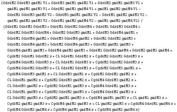
Approximating the tableau equations has reduced the transfer function, which was initially of order four, to the first-order formula we were looking for. In a last postprocessing step, we can remove all remaining numerically irrelevant terms by solution-based approximation.
In[45]:= dpcmos2 = GetDesignPoint[stacmoshf];
In[46]:= tfcmoshfSAG = Simplify @
ApproximateTransferFunction[tfcmoshf, s, dpcmos2, 0.1]
Out[52]= 
From the above result we can now easily compute a formula for the pole of the transfer function by solving the denominator of the expression for s:
In[47]:= Solve[Denominator[tfcmoshfSAG] == 0, s] // Simplify
Out[53]= 
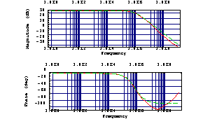
Finally, we verify the result by evaluating the approximated formula with the design-point values and comparing its frequency response to that of the original PSpice simulation. The simplified formula turns out to be a good approximation from DC up to a frequency of about  . .
In[48]:= tfcmoshf2 = Together[tfcmoshfSAG
/. dpcmos2 /. s -> 2 Pi I f]
Out[54]= 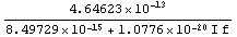
In[49]:= BodePlot[reference, {tfcmosPSpice[f], tfcmoshf2},
{f, 1., 1.*10^9}, ShowLegend -> False]
Out[55]= 
|