Wolfram 语言与系统参考资料中心

AsymptoticProduct

AsymptoticProduct[f,x,xx₀]

计算当 x 接近 x₀ 时，不定积的渐近逼近.

AsymptoticProduct[f,{x,a,b},αα₀]

计算当 α 接近 α₀ 时，定积的渐近逼近.

AsymptoticProduct[f,…,{ξ,ξ₀,n}]

计算阶数 n 的渐近逼近.

更多信息和选项

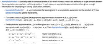
AsymptoticProduct 通常用于计算无法找到确切结果的乘积，或者用于获取计算、比较和诠释的更简单答案. 在这种情况下，渐近逼近通常会提供足够的信息来简化或解决应用问题.
AsymptoticProduct[f,…,ξξ₀] 计算 f 乘积的渐近展开式中的前导项. 使用 SeriesTermGoal 指定更多项.
如果精确结果为 g[x] 且在 x₀ 处阶数 n 的渐近逼近为 g_n[x]，那么，当 xx₀，则 AsymptoticLess[g[x]-g_n[x],g_n[x]-g_n-1[x],xx₀] 或g[x]-g_n[x]∈o[g_n[x]-g_n-1[x]].
渐近逼近 g_n[x] 经常以和 g_n[x]α_kϕ_k[x] 形式给出，其中，{ϕ₁[x],…,ϕ_n[x]} 是在 xx₀ 的一个渐近标度 ϕ₁[x]≻ϕ₂[x]≻⋯>ϕ_n[x]. 那么当 xx₀，则 AsymptoticLess[g[x]-g_n[x],ϕ_n[x],xx₀] 或 g[x]-g_n[x]∈o[ϕ_n[x]].
xx₀ 的泰勒尺度

xx₀ 的 Laurent 尺度

x±∞ 的 Laurent 尺度

xx₀ 的 Puiseux 尺度
用于表示渐近逼近的尺度是从问题中自动推断出，通常可以包括更多的奇异尺度.
中心 α₀ 可以是任何有限或无限的实数或复数.
阶数 n 必须为正整数，并指定渐近展开的近似阶数. 它与多项式次数无关.
可以给出以下选项：

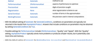
AccuracyGoal	Automatic	寻求绝对精度的位数
Assumptions	$Assumptions	关于参数的假设
GenerateConditions	Automatic	是否产生包含参数条件的答案
GeneratedParameters	None	如何命名生成的参数
Method	Automatic	使用的方法
PerformanceGoal	$PerformanceGoal	性能方面的优化
PrecisionGoal	Automatic	寻求精度的位数
Regularization	None	使用何种正则化方案
SeriesTermGoal	Automatic	逼近中的项数
WorkingPrecision	Automatic	内部计算中使用的精度

对于 GenerateConditions，默认设置为 Automatic，则通常不会在 AsymptoticProduct 的结果中返回参数的条件. 可以通过将 GenerateConditions 设为 True 来获得包含参数条件的答案.
PerformanceGoal 的可能设置包括 $PerformanceGoal、"Quality" 和 "Speed". 当使用 "Quality" 设置，AsymptoticProduct 通常可以解决更多问题或产生更简单的结果，但是它可能会占用更多的时间和内存.
当 WorkingPrecision、AccuracyGoal 和 PrecisionGoal 的默认设置为 Automatic，即使输入具有无限精度，AsymptoticProduct 也会以较低的精度返回渐近逼近.

范例

打开所有单元关闭所有单元

基本范例 (2)

计算乘积的渐近逼近:

Wolfram Language code: AsymptoticProduct[k, {k, 2, n}, n -> ∞]

与确切值进行比较：

Wolfram Language code: {% /. {n -> 20.}, Product[k, {k, 2, 20}]//N}

使用 SeriesTermGoal 改善逼近:

Wolfram Language code: AsymptoticProduct[k, {k, 2, n}, n -> ∞, SeriesTermGoal -> 2]

Wolfram Language code: % /. {n -> 20.}

根据参数计算乘积的渐近展开：

Wolfram Language code: f[a_] := (k^2 - 1/k^2 + a)

Wolfram Language code: DiscretePlot[Product[f[0.02], {k, 2, n}], {n, 5, 40}, PlotStyle -> Red]

计算所需的扩展：

Wolfram Language code: AsymptoticProduct[f[a], {k, 2, ∞}, {a, 0, 2}]

与小 a 的确切值进行比较：

Wolfram Language code: {% /. {a -> 0.02}, Product[f[0.02], {k, 2, ∞}]}

范围 (14)

基本用途 (3)

计算一个不定乘积的渐近逼近：

Wolfram Language code: AsymptoticProduct[k ^ 2, k, {k, ∞, 2}]

计算定积的渐近逼近：

Wolfram Language code: AsymptoticProduct[(k ^ 2 + 1) / (k ^ 2 - 2), {k, 1, n}, {n, ∞, 2}]

计算参数乘积的渐近逼近:

Wolfram Language code: AsymptoticProduct[k + m, {k, 1, n}, m -> 0]

不定乘积 (5)

计算多项式乘积的渐近展开式：

Wolfram Language code: AsymptoticProduct[(k + 1)k, k, {k, ∞, 2}]//Together

比较由 Product 给出的结果：

Wolfram Language code: Product[(k + 1)k, k]

Wolfram Language code: Series[%, {k, ∞, 2}]//Normal//Together

有理函数的不定乘积的渐近展开：

Wolfram Language code: AsymptoticProduct[1 / (k + 3), k, {k, ∞, 3}]

Wolfram Language code: AsymptoticProduct[(k ^ 2 + 1) / (k ^ 2 - 2), k, {k, ∞, 5}]

超几何项的不定乘积的渐近展开：

Wolfram Language code: AsymptoticProduct[k k!, k, {k, ∞, 2}]

估算一个点的值：

Wolfram Language code: (% /. k -> 21.) / (% /. k -> 1.)

与 NProduct 给出的值进行比较：

Wolfram Language code: NProduct[k k!, {k, 1, 20}]

有理指数函数的不定乘积的渐近展开：

Wolfram Language code: AsymptoticProduct[E ^ (-k) / (k + 2), k, {k, ∞, 2}]

代数函数的不定乘积的渐近展开：

Wolfram Language code: AsymptoticProduct[(k ^ (13 / 4) - 1) / (k ^ (13 / 4) + 1), k, {k, ∞, 3}]

定积 (4)

计算有理乘积的渐近展开：

Wolfram Language code: AsymptoticProduct[(k ^ 2 + 3) / (k ^ 2 - 3), {k, 3, n}, {n, ∞, 2}]

Wolfram Language code: DiscretePlot[Product[(k ^ 2 + 3) / (k ^ 2 - 3), {k, 3, n}], {n, 4, 50}]

与 NProduct 给出的结果进行比较：

Wolfram Language code: %% /. {n -> 30.`20}//N//Chop

Wolfram Language code: NProduct[(k ^ 2 + 3) / (k ^ 2 - 3), {k, 3, 30}]

有理指数积的渐近逼近：

Wolfram Language code: AsymptoticProduct[E ^ (-k)k ^ 2 / (k + 1), {k, 1, n - 1}, {n, ∞, 1}]

与 NProduct 给出的结果进行比较：

Wolfram Language code: % /. {n -> 20.`20}

Wolfram Language code: NProduct[E ^ (-k)k ^ 2 / (k + 1), {k, 1, 19}]

计算超几何积的渐近逼近：

Wolfram Language code: AsymptoticProduct[k! k ^ 2, {k, 1, n}, n -> ∞]//Simplify

与精确结果进行比较：

Wolfram Language code: % /. n -> 100.`20//Chop

Wolfram Language code: Product[k! k ^ 2, {k, 1, n}] /. {n -> 100.}

代数乘积的渐近展开：

Wolfram Language code: AsymptoticProduct[(k ^ (13 / 4) - 1) / (k ^ (13 / 4) + 1), {k, 2, n}, {n, ∞, 3}]

与精确结果进行比较：

Wolfram Language code: % /. {n -> 80}

Wolfram Language code: Product[(k ^ (13 / 4) - 1) / (k ^ (13 / 4) + 1), {k, 2., 50}]

参数乘积 (2)

有限积关于参数 a 的渐近展开：

Wolfram Language code: AsymptoticProduct[ k + a, {k, 1, n}, {a, 0, 2}]//FullSimplify

计算数值近似值：

Wolfram Language code: % /. {a -> 0.03, n -> 200}//N

与 NProduct 给出的结果进行比较：

Wolfram Language code: NProduct[k + 0.03, {k, 1, 200}]

Wolfram Language code: (% - %%) / % * 100

无限积相对于参数 z 的渐近展开：

Wolfram Language code: AsymptoticProduct[1 - z ^ 2 / ( i ^ 2), {i, 1, ∞}, {z, 0, 2}]

计算数值近似值：

Wolfram Language code: % /. {z -> 0.13}

与 NProduct 给出的结果进行比较：

Wolfram Language code: NProduct[1 - 0.13 ^ 2 / ( i ^ 2), {i, 1, ∞}]

通过计算更多项来改进渐近逼近：

Wolfram Language code: AsymptoticProduct[1 - z ^ 2 / ( i ^ 2), {i, 1, ∞}, {z, 0, 4}]

Wolfram Language code: % /. {z -> 0.13}

应用 (4)

计算有限积的近似值：

Wolfram Language code: AsymptoticProduct[(k ^ 2 + 4) / (k ^ 2 + 1), {k, 1, n}, {n, ∞, 3}]

计算 n 增加的数值近似：

Wolfram Language code: Table[%, {n, {5, 10, 300}}]//N[#, 20]&//N//Chop

与 Product 给出的精确结果进行比较：

Wolfram Language code: Table[Product[(k ^ 2 + 4) / (k ^ 2 + 1), {k, 1, n}], {n, {5, 10, 300}}]//N[#, 20]&//N//Chop

与精确的符号公式的级数展开比较：

Wolfram Language code: Product[(k ^ 2 + 4) / (k ^ 2 + 1), {k, 1, n}]

Wolfram Language code: Series[%, {n, ∞, 3}]//Normal

使用相应有限积的渐近展开来计算无限有理积的值：

Wolfram Language code: fp = AsymptoticProduct[(i ^ 3 - 1) / (i ^ 3 + 1), {i, 2, n}, {n, ∞, 2}]

获得无限积的值：

Wolfram Language code: fp /. {n -> ∞}

使用 DiscreteLimit 获得相同的答案：

Wolfram Language code: DiscreteLimit[Product[(i ^ 3 - 1) / (i ^ 3 + 1), {i, 2, n}], n -> ∞]

使用 Product 确认答案：

Wolfram Language code: Product[(i ^ 3 - 1) / (i ^ 3 + 1), {i, 2, ∞}]

通过计算相应的不定积的渐近展开来建立无限积的收敛：

Wolfram Language code: AsymptoticProduct[(3i ^ 2 + 5) / (3i ^ 2 + 1), i, i -> ∞]

使用有限积的渐近展开来计算精确值：

Wolfram Language code: AsymptoticProduct[(3i ^ 2 + 5) / (3i ^ 2 + 1), {i, 1, n}, n -> Infinity]

使用 Product 获取相同的结果：

Wolfram Language code: Product[(3i ^ 2 + 5) / (3i ^ 2 + 1), {i, 1, ∞}]

计算的渐近逼近：

Wolfram Language code: asy = 2 AsymptoticProduct[(4 k ^ 2) / ((2 k - 1) (2 k + 1)), {k, 1, n}, {n, ∞, 3}]//Expand

Wolfram Language code: Table[asy, {n, 1000, 10000, 2000}]//N

计算渐近表达式的极限值：

Wolfram Language code: DiscreteLimit[asy, n -> ∞]

可视化极限值的收敛：

Wolfram Language code: DiscretePlot[asy, {n, 1000, 10000, 500}]

属性和关系 (4)

AsymptoticProduct 计算给定阶的积：

Wolfram Language code: asym = AsymptoticProduct[k, {k, 1, n}, {n, ∞, 2}]//Simplify

Wolfram Language code: exact = n!;

Wolfram Language code: Series[asym - exact, {n, ∞, 2}]//Normal//FullSimplify

使用 Product 计算闭式积：

Wolfram Language code: AsymptoticProduct[1 / (k ^ 2 - 1), {k, 2, n}, {n, ∞, 2}]

Wolfram Language code: Product[1 / (k ^ 2 - 1), {k, 2, n}]

Wolfram Language code: Series[% - %%, {n, ∞, 2}]//Normal//Simplify

使用 NProduct 计算数值近似：

Wolfram Language code: AsymptoticProduct[1 / k ^ 2, {k, 1, n}, {n, ∞, 2}]

Wolfram Language code: % /. {n -> 40.`20}//N

Wolfram Language code: NProduct[1 / k ^ 2, {k, 1, 40}]

计算乘积的渐近近似：

Wolfram Language code: AsymptoticProduct[(k ^ (5 / 4) - 1) / (k ^ (5 / 4) + 1), k, k -> ∞]

使用 DiscreteAsymptotic 获取同样的结果：

Wolfram Language code: Product[(k ^ (5 / 4) - 1) / (k ^ (5 / 4) + 1), k]

Wolfram Language code: DiscreteAsymptotic[%, k -> ∞]

Top

更多学习资源

技术支持

数据科学、金融与商业

工程

科学与技术

教育科技

教育举措

开始

提高你的技能

与我们合作

成人教育计划

青少年教育计划

欢迎阅读

AsymptoticProduct

更多信息和选项

范例

基本范例 (2)

范围 (14)

基本用途 (3)

不定乘积 (5)

定积 (4)

参数乘积 (2)

应用 (4)

属性和关系 (4)

文本

CMS

APA

BibTeX

BibLaTeX

		xx₀ 的泰勒尺度
		xx₀ 的 Laurent 尺度
		x±∞ 的 Laurent 尺度
		xx₀ 的 Puiseux 尺度

AsymptoticProduct

更多信息和选项

范例

基本范例 (2)

范围 (14)

基本用途 (3)

不定乘积 (5)

定积 (4)

参数乘积 (2)

应用 (4)

属性和关系 (4)

参见

相关指南

历史

文本

CMS

APA

BibTeX

BibLaTeX