创建阶数为 n 的第一类切比雪夫低通滤波器.
Chebyshev1FilterModel[{n,ωc}]
使用截止频率 ωc.
Chebyshev1FilterModel[{"type",spec}]
使用指定参数 spec 设计已知 "type" 的滤波器.
Chebyshev1FilterModel[{"type",spec},var]
以变量 var 的形式表示模型.
Chebyshev1FilterModel
创建阶数为 n 的第一类切比雪夫低通滤波器.
Chebyshev1FilterModel[{n,ωc}]
使用截止频率 ωc.
Chebyshev1FilterModel[{"type",spec}]
使用指定参数 spec 设计已知 "type" 的滤波器.
Chebyshev1FilterModel[{"type",spec},var]
以变量 var 的形式表示模型.
更多信息
- Chebyshev1FilterModel 以 TransferFunctionModel 返回滤波器.
- Chebyshev1FilterModel[{n,ω}] 返回频率 ω 处衰减量为

(约为 3dB)的低通滤波器. - Chebyshev1FilterModel[n] 的截至频率为 1.
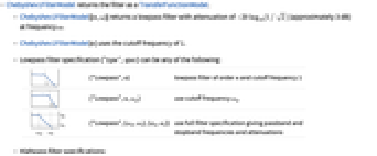
- 低通滤波器规范 {"type",spec} 可以是下面所列的任何一种:
-
{"Lowpass",n} 阶数为 n、截止频率为 1 的低通滤波器 
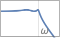
{"Lowpass",n,ωp} 截至频率为 ωp 
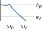
{"Lowpass",{ωp,ωs},{ap,as}} 使用完整的滤波器规范(给出通带和阻带的截至频率和衰减) - 高通滤波器规范:
-
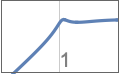
{"Highpass",n} 截止频率为 1 的高通滤波器 
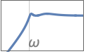
{"Highpass",n,ωp} 截至频率为 ωp 
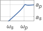
{"Highpass",{ωs,ωp},{as,ap}} 完整的滤波器规范 - 带通滤波器规范:
-
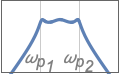
{"Bandpass",n,{ωp1,ωp2}} 通带频率为 ωp1 和 ωp2 的带通滤波器 
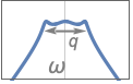
{"Bandpass",n,{{ω,q}}} 中心频率为 ω,品质因数为 q 
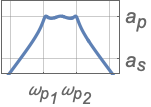
{"Bandpass",{ωs1,ωp1,ωp2,ωs2},{as,ap}} 完整的滤波器规范 - 带阻滤波器规范:
-
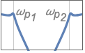
{"Bandstop",n,{ωp1,ωp2}} 通带频率为 ωp1 和 ωp2 的带阻滤波器 
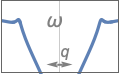
{"Bandstop",n,{{ω,q}}} 中心频率为 ω,品质因数为 q 
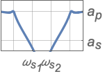
{"Bandstop",{ωp1,ωs1,ωs2,ωp2},{ap,as}} 完整的滤波器规范 - 频率值应该以升序给出.
- 值 ap 和 as 分别是带通和带阻衰减量的绝对值.
- 已知增益
,衰减量为
. - 品质因数 q 的定义为
,其中 ω 是带通或带阻滤波器的中心频率. q 的值越高,滤波器越窄.
范例
打开所有单元 关闭所有单元基本范例 (2)
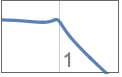
tf = Chebyshev1FilterModel[3]tf = Chebyshev1FilterModel[3, s]BodePlot[tf, GridLines -> Automatic, PlotLayout -> "Magnitude"]tf = Chebyshev1FilterModel[{"Lowpass", {1., 2.}, {1., 20.}}, s]//ChopPlot[Abs[tf[I * ω]], {ω, 0, 3}, PlotRange -> All, Epilog -> {Pink, Dashed, Line[{{0, 0.89}, {1, 0.89}, {1, 0.1}}], Line[{{2., 0.89}, {2., 0.1}, {3., 0.1}}]}]范围 (5)
Chebyshev1FilterModel[{2, ω}, s]//NChebyshev1FilterModel[{2, 1}, s]Chebyshev1FilterModel[{2, N[1, 24]}, s]BodePlot[Chebyshev1FilterModel[{"Highpass", {1., 2.}, {20., 1.}}], GridLines -> Automatic, PlotLayout -> "Magnitude"]BodePlot[Chebyshev1FilterModel[{"Bandpass", 3, {1, 10}}], {0.1, 100}, GridLines -> Automatic, PlotLayout -> "Magnitude"]BodePlot[Chebyshev1FilterModel[{"Bandpass", 3, {{1, 1 / 3}}}], {0.01, 100}, GridLines -> Automatic, PlotLayout -> "Magnitude"]tf = Chebyshev1FilterModel[{"Bandpass", {0.1, 1., 10., 100.}, {60, -20Log10[1 / Sqrt[2]]}}];BodePlot[tf, {0.1, 100}, GridLines -> Automatic, PlotLayout -> "Magnitude"]创建一个带阻滤波器,其通带频率为 1 和 10,衰减阶数为 3:
BodePlot[Chebyshev1FilterModel[{"Bandstop", 3, {1, 10}}], {0.1, 100}, GridLines -> Automatic, PlotLayout -> "Magnitude"]BodePlot[Chebyshev1FilterModel[{"Bandstop", 3, {{1, 1 / 3}}}], {0.01, 100}, GridLines -> Automatic, PlotLayout -> "Magnitude"]tf = Chebyshev1FilterModel[{"Bandstop", {0.1, 1., 10., 100.}, {1, 20}}];
BodePlot[tf, {0.01, 1000.}, GridLines -> Automatic, PlotLayout -> "Magnitude"]应用 (5)
tf = Chebyshev1FilterModel[{"Lowpass", {1., 2.}, {1, 40}}];ω = 1 / 5;input = (Sin[ω t] + 1 / 2 Sin[25ω t]) UnitStep[t];
response1 = OutputResponse[tf, input, {t, 0, 100}][[1]];第一类切比雪夫滤波器把响应的相位平移了 Arg[tf[ω ]],其中 ω 是输入正弦波的频率:
Plot[{input, response1}, {t, 20, 100}]delay = Arg[tf[I ω]] / ω//First//First;
Plot[Evaluate[Flatten[{input, response1 /. t -> (t - delay)}]], {t, 20, 100}]tf2 = TransferFunctionTransform[1 / #&, tf];Plot[Evaluate[Flatten[{input, OutputResponse[tf2, input, {t, 0, 100}]}]], {t, 20, 100}]用 Chebyshev 1 型近似设计一个数字低通滤波器,满足以下通带和阻带频率以及衰减要求:
Subscript[ω, p] = 0.4π;Subscript[ω, s] = 0.6π;
Subscript[a, p] = 1;Subscript[a, s] = 20;{Subscript[Ω, p] = 2 Tan[(0.4π/2)], Subscript[Ω, s] = 2 Tan[(0.6π/2)]}tf = Chebyshev1FilterModel[{"Lowpass", {Subscript[Ω, p], Subscript[Ω, s]}, {Subscript[a, p], Subscript[a, s]}}, s]dtf = ToDiscreteTimeModel[tf, 1, z]//ChopBodePlot[dtf, {0.1 π, π}, PlotLayout -> "Magnitude", GridLines -> {{Subscript[ω, p], Subscript[ω, s]}, {10^-Subscript[a, p] / 20, 10^-Subscript[a, s] / 20}}, ScalingFunctions -> {"Linear", "Absolute"}, PlotRange -> All]创建可以近似离散时间切比雪夫 1 型 IIR 滤波器的长度为 31 的 FIR 滤波器:
OutputResponse[dtf, KroneckerDelta[n], {n, 0, 30}]//ChopListPlot[%, PlotRange -> All, Filling -> 0]data = Transpose[FinancialData["GE", {"Jan. 1, 2012", "Jan. 1, 2013"}]["Path"]];
fir = OutputResponse[ToDiscreteTimeModel[Chebyshev1FilterModel[{3, 1.}], 1], KroneckerDelta[n], {n, 0, 40}]//Chop//Flatten;
DateListPlot[{Transpose[data], Transpose[{data[[1]], -ListConvolve[fir, data[[2]], 4]}]}, PlotRange -> All, PlotLegends -> {"original", "smoothed"}]h = ToDiscreteTimeModel[Chebyshev1FilterModel[{"Lowpass", 3, 0.75}], 1];
RecurrenceFilter[h, [image]]h = ToDiscreteTimeModel[Chebyshev1FilterModel[{"Highpass", 3, 0.75}], 1];
RecurrenceFilter[h, [image]]属性和关系 (8)
tf = Chebyshev1FilterModel[{"Lowpass", #}]& /@ {1, 2, 3};
BodePlot[tf, {0.1, 10}, GridLines -> Automatic, PlotLayout -> "Magnitude", PlotLegends -> {1, 2, 3}]"Bandpass" 滤波器的通带宽度随品质因数 q 的增加而减小:
tf = Chebyshev1FilterModel[{"Bandpass", 2, {{1, #}}}]& /@ {0.5, 1., 3.};
BodePlot[tf, {0.1, 10}, GridLines -> Automatic, PlotLayout -> "Magnitude", PlotRange -> {0, -80}, PlotLegends -> {0.5, 1., 3.}]BodePlot[Chebyshev1FilterModel[{"Lowpass", 3}], {0.1, 10.}, PlotLayout -> "Phase", GridLines -> Automatic]BodePlot[Chebyshev1FilterModel[{"Lowpass", #}]& /@ {1, 2, 3}, {0.1, 10.}, PlotLayout -> "Phase", GridLines -> Automatic, PlotLegends -> {1, 2, 3}]BodePlot[Chebyshev1FilterModel[{"Bandpass", 2, {{1, #}}}]& /@ {1., 3., 5.}, {0.1, 10}, GridLines -> Automatic, PlotLayout -> "Phase", PlotLegends -> {1., 3., 5.}]t1 = Chebyshev1FilterModel[{"Lowpass", {1., 2.}, {1., 20.}}, s]t2 = Chebyshev2FilterModel[{"Lowpass", {1., 2.}, {1., 20.}}, s]Plot[{Abs[t1[I * ω]], Abs[t2[I * ω]]}, {ω, 0, 3}, PlotRange -> All, Epilog -> {Pink, Dashed, Line[{{0, 0.89}, {1, 0.89}, {1, 0.1}}], Line[{{2., 0.89}, {2., 0.1}, {3., 0.1}}]}]SystemsModelOrder[StateSpaceModel[Chebyshev1FilterModel[{"Lowpass", {1., 2.}, {1., 20.}}]]]tfm = Chebyshev1FilterModel[11];
poles = TransferFunctionPoles[tfm]PoleZeroPlot[tfm, ...]dtf = ToDiscreteTimeModel[Chebyshev1FilterModel[11], 1]poles = TransferFunctionPoles[dtf];
ListPlot[{Re[#], Im[#]}& /@ poles[[1, 1]], PlotRange -> {{-1, 1}, {-1, 1}}, PlotStyle -> PointSize[Large], Epilog -> {Dotted, Circle[]}, AspectRatio -> 1]lo = Chebyshev1FilterModel[3];
hi = TransferFunctionTransform[(1 / #&), lo];BodePlot[{lo, hi}, {0.1, 10}, GridLines -> Automatic, PlotLayout -> "Magnitude"]相关指南
-
▪
- 信号滤波与滤波器设计 ▪
- 图像计算:更新历史
文本
Wolfram Research (2012),Chebyshev1FilterModel,Wolfram 语言函数,https://reference.wolfram.com/language/ref/Chebyshev1FilterModel.html (更新于 2016 年).
CMS
Wolfram 语言. 2012. "Chebyshev1FilterModel." Wolfram 语言与系统参考资料中心. Wolfram Research. 最新版本 2016. https://reference.wolfram.com/language/ref/Chebyshev1FilterModel.html.
APA
Wolfram 语言. (2012). Chebyshev1FilterModel. Wolfram 语言与系统参考资料中心. 追溯自 https://reference.wolfram.com/language/ref/Chebyshev1FilterModel.html 年
BibTeX
@misc{reference.wolfram_2026_chebyshev1filtermodel, author="Wolfram Research", title="{Chebyshev1FilterModel}", year="2016", howpublished="\url{https://reference.wolfram.com/language/ref/Chebyshev1FilterModel.html}", note=[Accessed: 15-September-2026]}
BibLaTeX
@online{reference.wolfram_2026_chebyshev1filtermodel, organization={Wolfram Research}, title={Chebyshev1FilterModel}, year={2016}, url={https://reference.wolfram.com/language/ref/Chebyshev1FilterModel.html}, note=[Accessed: 15-September-2026]}