ConnectSystemModelComponents[{"c1"∈comp1,…},{"c1.a""c2.b",…}]
コンポーネント"c1"のコネクタ"a"をコンポーネント"c2"のコネクタ"b"と繋ぐという風に,システムのモデルを作る.
ConnectSystemModelComponents
ConnectSystemModelComponents[{"c1"∈comp1,…},{"c1.a""c2.b",…}]
コンポーネント"c1"のコネクタ"a"をコンポーネント"c2"のコネクタ"b"と繋ぐという風に,システムのモデルを作る.
詳細とオプション
- ConnectSystemModelComponentsはコンポーネントを組み立て新たなシステムモデルを作成する.この接続は値を伝達し,システム内に保存法則を設定する.
- ConnectSystemModelComponentsはSystemModel[…]を返す.
- ConnectSystemModelComponents["NewModel",…]は,"NewModel"という名前の作成されたモデルを返す.
- ConnectSystemModelComponents["PackageA.NewModel",…]は"PackageA"に"NewModel"を挿入する.
- compiは,SystemModelオブジェクト,モデルの完全名の文字列,あるいはSystemModelが許容するモデルの短縮名でよい.
- ConnectSystemModelComponents[…,spec]の spec は次のキーを持つAssociationである.
-
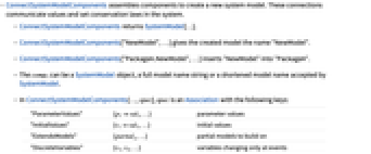
"ParameterValues" {p1val1,…} パラメータ値 "InitialValues" {v1val1,…} 初期値 "ExtendsModels" {partial1,…} 構築する部分モデル "DiscreteVariables" {v1,v2,…} イベントについてのみ変化する変数 "SimulationSettings" {opt1val1,…} モデルのシミュレーションオプション - ConnectSystemModelComponents[…,"ExtendsModels"partial]のときは,新規モデルがModelica内で定義されている既存 partial SystemModelに結合される. »
- "ExtendsModels"{"partial1",…}を使ってモデルを複数のモデルに拡張することができる.
- 上に構築する部分モデルは,大抵の場合,Interfacesパッケージで定義されている.例えば,SystemModels["Modelica.Electrical.Analog.Interfaces.*","model"|"block"]を使って組込みの電気ライブラリにある部分モデルを探すことができる.
- "InitialValues"はModelicaモデルの start 特性に対応する.
- 次は,"SimulationsSettings"->{opt1val1,…}で使用可能なオプションである.
-
"Method" シミュレーションメソッド "StartTime" シミュレーションの開始時間 "StopTime" シミュレーションの終了時間 - 次は,使用可能な適応的ステップ"Method"の値である.
-
"DASSL" DASSL DAEソルバ "CVODES" CVODES ODEソルバ - 次は,適応的ステップ法のオプションである.
-
"InterpolationPoints" 補間点の数 "Tolerance" 適応的ステップサイズの許容範囲 - 次は,使用可能な固定ステップ"Method"の値である.
-
"Euler" 次数1の明示的なオイラー(Euler)法 "Heun" 次数2のホイン(Heun)法 "RungeKutta" 次数4の明示的なルンゲ・クッタ(Runge–Kutta)法 - 次は,固定ステップ法のオプションである.
-
"StepSize" 固定ステップサイズ - 作成されたモデルの線図のレイアウトはGraphLayoutオプションで制御できる.
例題
すべて開く すべて閉じる例 (2)
components = {"L"∈"Modelica.Electrical.Analog.Basic.Inductor", "AC"∈"Modelica.Electrical.Analog.Sources.SineVoltage", "G"∈"Modelica.Electrical.Analog.Basic.Ground"};connections = {"G.p" -> "AC.n", "AC.p" -> "L.n", "L.p" -> "AC.n"};model = ConnectSystemModelComponents[components, connections]SystemModelPlot[model, {"L.i", "L.v"}, 5]Modelica.Blocks内のAbsとSineのコンポーネントを参照するのに短縮名を使う:
comp = {"a"∈"Math.Abs", "sine"∈"Sources.Sine"};conn = {"sine.y" -> "a.u"};model = ConnectSystemModelComponents[comp, conn]SystemModelPlot[model, {"a.y"}, 2]スコープ (5)
comp = {"sine"∈"Modelica.Blocks.Sources.Sine", "sample"∈"Discrete.Sampler"};conn = {"sine.y""sample.u"};model = ConnectSystemModelComponents[comp, conn]サンプリングされた信号のシミュレーションを行い,プロットする:
SystemModelPlot[model, {"sample.y"}, 2]comp = {"inAdd"∈"DocumentationExamples.Basic.InputAdd", "cSource"∈"Modelica.Blocks.Sources.Constant"};conn = {"cSource.y""inAdd.u"};model = ConnectSystemModelComponents[comp, conn, <|"ParameterValues" -> {"inAdd.sine.amplitude" -> 3}|>]SystemModelPlot[model, {"inAdd.y"}, 2]comp = {"mass1"∈"HeatCapacitor", "mass2"∈"HeatCapacitor", "conduction"∈"ThermalConductor"};conn = {"mass1.port""conduction.port_a", "conduction.port_b""mass2.port"};model = ConnectSystemModelComponents[comp, conn]model2 = SystemModel[model, {"conduction.G" -> 10, "mass1.C" -> 15, "mass2.C" -> 40, "mass1.T" -> 373.15, "mass2.T" -> 273.15}];SystemModelPlot[model2, {"mass1.T", "mass2.T"}, 5]comp = {"fixed"∈"Modelica.Mechanics.Translational.Components.Fixed", "spring"∈"Modelica.Mechanics.Translational.Components.Spring", "mass"∈"Modelica.Mechanics.Translational.Components.Mass"};conn = {"fixed.flange""spring.flange_a", "spring.flange_b""mass.flange_a"};model = ConnectSystemModelComponents[comp, conn, <|"InitialValues" -> {"mass.s" -> 2}|>]SystemModelPlot[model, {"mass.s"}, 10]comp = {"world"∈"Modelica.Mechanics.MultiBody.World", "rev"∈"Modelica.Mechanics.MultiBody.Joints.Revolute", "damper"∈"Modelica.Mechanics.Rotational.Components.Damper", "body"∈"Modelica.Mechanics.MultiBody.Parts.Body"};conn = {"world.frame_b""rev.frame_a", "damper.flange_b""rev.axis", "rev.support""damper.flange_a", "body.frame_a""rev.frame_b"};model = ConnectSystemModelComponents[comp, conn, <|"ParameterValues" -> {"rev.useAxisFlange" -> True, "body.r_CM" -> {1, 0, 0}, "damper.d" -> 0.1}|>]振り子の経路のシミュレーションを行い,アニメーションにする:
sim = SystemModelSimulate[model, 10];graphics = sim["Graphics3D", t];pendulum[x_ ? NumberQ] := pendulum[x] = Show[graphics /. t -> x, PlotRange -> {{-1.2, 1.2}, {-1.2, 0.1}, {-.2, .2}}, ImageSize -> 300]Animate[Evaluate[pendulum[x]], {x, 0, 10}, AnimationRate -> 0.5, AnimationRunning -> False, SaveDefinitions -> True, TrackedSymbols :> {pendulum, x, graphics}]一般化と拡張 (1)
接続には,Rule,DirectedEdge,UndirectedEdgeが使える:
comp1 = {"sine"∈"Modelica.Blocks.Sources.Sine", "sample"∈"ZeroOrderHold"};Ruleを使って接続を指定する:
conn1 = {"sine.y" -> "sample.u"};model1 = ConnectSystemModelComponents[comp1, conn1]DirectedEdgeとUndirectedEdgeを使って接続を指定する:
comp2 = Append[comp1, "foh"∈"FirstOrderHold"];conn2 = {"sine.y""sample.u", "sample.y""foh.u"};model2 = ConnectSystemModelComponents[comp2, conn2]Column[{SystemModelPlot[model1, {"sample.y"}, 2], SystemModelPlot[model2, {"foh.y"}, 2]}]オプション (3)
GraphLayout (3)
GraphLayoutを使ってモデルの線図のレイアウトが指定できる:
comp = {"sine"∈"Modelica.Blocks.Sources.Sine", "sample"∈"ZeroOrderHold", "foh"∈"FirstOrderHold"};conn = {"sine.y""sample.u", "sample.y""foh.u"};ConnectSystemModelComponents[comp, conn, GraphLayout -> "LinearEmbedding"]デフォルトで,"SpringElectricalEmbedding"で重みが付けられた辺が使われる:
comp = {"sine"∈"Modelica.Blocks.Sources.Sine", "sample"∈"ZeroOrderHold"};conn = {"sine.y" -> "sample.u"};ConnectSystemModelComponents[comp, conn, GraphLayout -> {"SpringElectricalEmbedding", "EdgeWeighted" -> True}]comp = {"sine"∈"Modelica.Blocks.Sources.Sine", "sample"∈"ZeroOrderHold"};conn = {"sine.y" -> "sample.u"};ConnectSystemModelComponents[comp, conn, GraphLayout -> None]アプリケーション (3)
DCモーター (1)
電気コンポーネントと力学コンポーネントを接続してDCモーターのモデルを作る:
components = {"step1"∈"Blocks.Sources.Step", "resistor1"∈"Analog.Basic.Resistor", "inductor1"∈"Analog.Basic.Inductor", "EMF1"∈"RotationalEMF", "ground1"∈"Analog.Basic.Ground", "signalVoltage1"∈"Analog.Sources.SignalVoltage", "inertia1"∈"Rotational.Components.Inertia"};connections = {"resistor1.n""inductor1.p", "inductor1.n""EMF1.p", "step1.y""signalVoltage1.v", "signalVoltage1.p""resistor1.p", "EMF1.n""signalVoltage1.n", "ground1.p""signalVoltage1.n", "EMF1.flange""inertia1.flange_a"};model = ConnectSystemModelComponents[components, connections]SystemModelPlot[model, "inertia1.w", 10]ローパスフィルタ (1)
a = LeastSquaresFilterKernel[{"Lowpass", 0.1}, 20];h = ListZTransform[a, z];tf = TransferFunctionModel[h, z, SamplingPeriod -> 0.01]//TransferFunctionCancellowPass = CreateSystemModel[tf];signal = CreateSystemModel["Signal", {y[t] == Abs[Sin[t Cos[2t]]]t}, t, <|"ExtendsModels" -> "Modelica.Blocks.Interfaces.SignalSource"|>];model = ConnectSystemModelComponents["FilteredSignal", {"signal"∈signal, "filter"∈lowPass}, {"signal.y""filter.u"}]信号出力とフィルタをかけられた信号のシミュレーションを行い,プロットする:
sim = SystemModelSimulate[model, 10];SystemModelPlot[sim, {"signal.y", "filter.y"}]イナータ (1)
相対加速度に比例する端子における力で,イナータ(inerter)を作る:
inerter = CreateSystemModel["Inerter", {f[t] == b(Subscript[v, rel]'[t])}, t, <|"ExtendsModels" -> "Translational.Interfaces.PartialCompliantWithRelativeStates"|>];減衰系にイナータを加えることで振動にどのような影響が出るかを比較する:
comp = {"damper"∈"Modelica.Mechanics.Translational.Components.Damper", "mass"∈"Modelica.Mechanics.Translational.Components.Mass", "force"∈"Modelica.Mechanics.Translational.Sources.Force", "vibration"∈"Interfaces.RealInput", "fixed"∈"Modelica.Mechanics.Translational.Components.Fixed", "spring"∈"Modelica.Mechanics.Translational.Components.Spring"};conn = {"fixed.flange" -> "spring.flange_a", "fixed.flange" -> "damper.flange_a", "damper.flange_b" -> "mass.flange_a", "spring.flange_b" -> "mass.flange_a", "force.flange" -> "mass.flange_a", "vibration" -> "force.f"};damping = ConnectSystemModelComponents[comp, conn]inerterDamping = ConnectSystemModelComponents[Append[comp, "inerter"∈inerter], Join[conn, {"inerter.flange_b" -> "mass.flange_a", "inerter.flange_a" -> "fixed.flange"}]]パラメータ値を設定し,正弦振動力で系のシミュレーションを行う:
d = 300;b = 700;c = 275;m = 2000;vibr = Function[t, Sin[10t]];tstop = 50;simInerter = SystemModelSimulate[inerterDamping, tstop, <|"Inputs" -> {"vibration" -> vibr}, "ParameterValues" -> {"inerter.b" -> b, "damper.d" -> d, "spring.c" -> c, "mass.m" -> m}|>];simDamper = SystemModelSimulate[damping, tstop, <|"Inputs" -> {"vibration" -> vibr}, "ParameterValues" -> {"damper.d" -> d, "spring.c" -> c, "mass.m" -> m}|>];SystemModelPlot[{simInerter, simDamper}, {"mass.s"}, PlotLegends -> {"Inerter", "No inerter"}]減衰コンポーネントに対して働く力は,イナータによって劇的に減少している:
damperForceInerter = simInerter[{"damper.f"}]//First;damperForce = simDamper[{"damper.f"}]//First;Plot[{Abs[damperForceInerter[t]], Abs[damperForce[t]]}, {t, 0, 10}, PlotLegends -> {"Inerter", "No inerter"}]特性と関係 (3)
CreateSystemModelを使って微分方程式に基づいたモデルを作る:
model = CreateSystemModel[{Subscript[y, 1]'[t] == Subscript[y, 1][t] + Subscript[y, 2][t], Subscript[y, 2]'[t] == Subscript[y, 1][t] + Sin[t]}, t];SystemModelPlot[{model, 2.5}, {"y_1", "y_2"}]CreateSystemModelはConnectSystemModelComponentsと同じように使うことができる:
model = CreateSystemModel[{"sine.y""sample.u"}, t, {"sine"∈"Modelica.Blocks.Sources.Sine", "sample"∈"ZeroOrderHold"}];SystemModelPlot[{model, 2}, {"sample.y"}]既存のコンポーネントに基づいた階層モデルを使うと,より大きい系が短時間で作成できる:
components = {"controller"∈"Systems.Components.LQControlSystem", "gear"∈"Systems.Components.GearBox", "motor"∈"Systems.Components.ElectricalMotor", "pendulum"∈"Systems.Components.Pendulum"};connections = {"pendulum.angle""controller.angle", "pendulum.position""controller.xPos", "motor.flange""gear.flange_a", "gear.flange_b""pendulum.flange_a", "motor.u""controller.y"};model = ConnectSystemModelComponents[components, connections]複雑なマルチドメインシステムが,少しのコンポーネントで構築できる:
model["Summary"]おもしろい例題 (1)
g = HararyGraph[4, 13];{vlist, elist} = {VertexList[g], EdgeList[g]};{nv, ne} = Length /@ {vlist, elist};vcomp = Map["v" <> ToString[#]∈"HeatCapacitor"&, vlist];ecomp = Table["e" <> ToString[i]∈"ThermalConductor", {i, ne}];complist = Join[vcomp, ecomp];connlist = Join@@Table[With[{e = ToString /@ elist[[i]], is = ToString[i]}, {"v" <> e[[1]] <> ".port""e" <> is <> ".port_a", "v" <> e[[2]] <> ".port""e" <> is <> ".port_b"}], {i, ne}];m = ConnectSystemModelComponents["ThermalGraph", complist, connlist, GraphLayout -> None];SetSystemModel[m, Join[{"v1.T" -> 320}, Table["e" <> ToString[i] <> ".G" -> 10, {i, ne}], Table["v" <> ToString[i] <> ".C" -> 15, {i, nv}]]];モデルのシミュレーションを行い,温度を色で示してアニメーションを作る:
sim = SystemModelSimulate[m, 5];temps = Table[i -> ColorData["TemperatureMap"][Rescale[sim["v" <> ToString[i] <> ".T", t], {293, 297}]], {i, nv}];vgraph[x_ ? NumberQ] := vgraph[x] = Graph[vlist, elist, VertexStyle -> (temps /. t -> x), VertexSize -> 0.3]Animate[Evaluate[vgraph[x]], {x, 0, 5}, AnimationRate -> 0.5, SaveDefinitions -> True, AnimationRunning -> False]関連するガイド
関連リンク
テキスト
Wolfram Research (2018), ConnectSystemModelComponents, Wolfram言語関数, https://reference.wolfram.com/language/ref/ConnectSystemModelComponents.html (2020年に更新).
CMS
Wolfram Language. 2018. "ConnectSystemModelComponents." Wolfram Language & System Documentation Center. Wolfram Research. Last Modified 2020. https://reference.wolfram.com/language/ref/ConnectSystemModelComponents.html.
APA
Wolfram Language. (2018). ConnectSystemModelComponents. Wolfram Language & System Documentation Center. Retrieved from https://reference.wolfram.com/language/ref/ConnectSystemModelComponents.html
BibTeX
@misc{reference.wolfram_2026_connectsystemmodelcomponents, author="Wolfram Research", title="{ConnectSystemModelComponents}", year="2020", howpublished="\url{https://reference.wolfram.com/language/ref/ConnectSystemModelComponents.html}", note=[Accessed: 08-September-2026]}
BibLaTeX
@online{reference.wolfram_2026_connectsystemmodelcomponents, organization={Wolfram Research}, title={ConnectSystemModelComponents}, year={2020}, url={https://reference.wolfram.com/language/ref/ConnectSystemModelComponents.html}, note=[Accessed: 08-September-2026]}