DiscreteInputOutputModel[{g0,g1,…,gn-1},u]
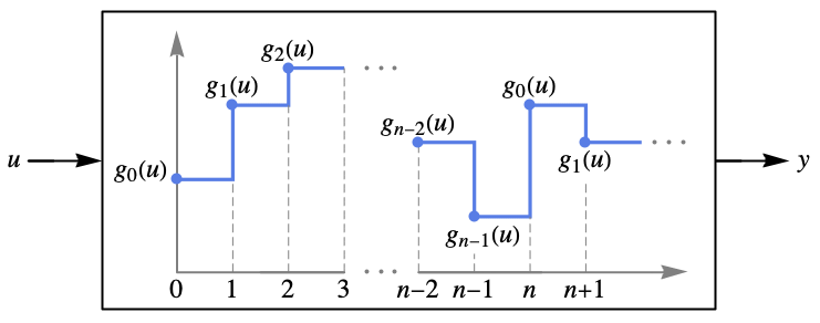
表示在采样时刻 i 输入为 u 和输出为
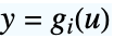
的离散时间模型.
DiscreteInputOutputModel[{g0,g1,…,gn-1},u,y]
可用于指定还依赖于输出变量 y 的输出
.
DiscreteInputOutputModel[…,{{u1,{…,u10}},…},{{y1,{…,y10}},…}]
指定每个信号在时刻 k<=0 时的输入和输出值.
DiscreteInputOutputModel
DiscreteInputOutputModel[{g0,g1,…,gn-1},u]
表示在采样时刻 i 输入为 u 和输出为
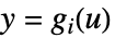
的离散时间模型.
DiscreteInputOutputModel[{g0,g1,…,gn-1},u,y]
可用于指定还依赖于输出变量 y 的输出
.
DiscreteInputOutputModel[…,{{u1,{…,u10}},…},{{y1,{…,y10}},…}]
指定每个信号在时刻 k<=0 时的输入和输出值.
更多信息和选项
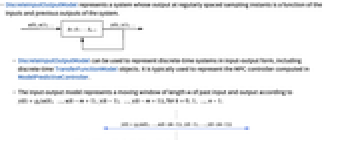
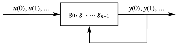
- DiscreteInputOutputModel 表示一个系统,在定期采样时刻的输出是系统输入和先前输出的函数.
- DiscreteInputOutputModel 可用于表示输入-输出形式的离散时间系统,包括离散时间 TransferFunctionModel 对象. 通常用于表示 ModelPredictiveController 中计算的 MPC 控制器.
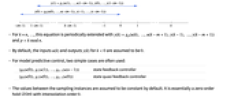
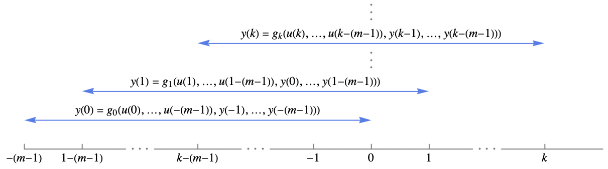
- 输入-输出模型表示过去的输入和输出组成的长度为 m 的移动窗口,

,其中
. - 对于 k=n,…,方程则被周期性地扩展为
,
. - 默认情况下,
时的输入
和输出
被视为
. - 对于模型预测控制,经常使用两种简单的情况:
-

状态反馈控制器 
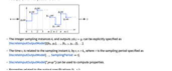
状态准反馈控制器 - 默认情况下,假定采样实例之间的值是恒定的. 实际上是一个插值阶数为 0 的零阶保持 (ZOH).
- 可用 DiscreteInputOutputModel[{{k0,g0},…,{kn-1,gn-1}},…] 明确指定整数采样实例 ki 和输出
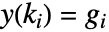
. - 时间 ti 与采样时刻 ki 之间的关系为 ti=τ ki,其中 τ 是采样周期,用 DiscreteInputOutputModel[…, SamplingPeriodτ] 指定.
- DiscreteInputOutputModel["prop"] 可用于计算属性.
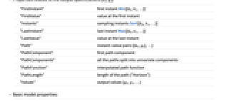
- 与输出规范 {ki,gi} 相关的属性:
-
"FirstInstant" 第一时刻 Min[{k0,k1,…}] "FirstValue" 第一时刻上的值 "Instants" 采样时刻 Sort[{k0,k1,…}] "LastInstant" 最后时刻 Max[{k0,k1,…}] "LastValue" 最后时刻上的值 "Path" “时刻-值”数据对 {{k0,g0},…} "PathComponent" 第一个路径分量 "PathComponents" 所有路径都拆分为单变量分量 "PathFunction" 插值路径函数 "PathLength" 路径的长度 ("Horizon") "Values" 输出的值 {g0,g1,…} - 基本的模型属性:
-
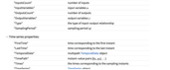
"InputsCount" 输入的数量 "InputVariables" 输入变量 u "OutputsCount" 输出的数量 "OutputVariables" 输出变量 y "Type" 输入-输出关系的类型 "SamplingPeriod" 采样周期 sp - 时间序列的属性:
-
"FirstTime" 对应于第一时刻的时间 "LastTime" 对应于最后时刻的时间 "TemporalData" 多路径 TemporalData 对象 "TimePath" “时刻-值”数据对 {{t0,g0},…} "Times" 对应于采样时刻的时间 "TimeSeries" TimeSeries 对象 "TimeValues" 采样时的输出值 - DiscreteInputOutputModel 接受以下选项:
-
MissingDataMethod None 处理缺失值的方法 ResamplingMethod {"Interpolation", InterpolationOrder0} 用于重采样路径的方法 SamplingPeriod Automatic 采样周期 
范例
打开所有单元 关闭所有单元基本范例 (3)
DiscreteInputOutputModel[{u[0], (u[0] + u[1]) / 2, (u[0] + u[1] + u[2]) / 3}, u]ListStepPlot[OutputResponse[%, RandomInteger[{-5, 5}, 50]]]DiscreteInputOutputModel[{u[0], u[1] - y[0], u[2] - y[1]}, u, y]ListStepPlot[OutputResponse[%, Table[Sin[t], {t, 0, 4π, 0.1}]]]DiscreteInputOutputModel[{u[0] + y[-1] + y[-2], u[1] + u[0] + u[-1]}, {{u, {-2, -1, 1}}}, {{y, {-1, -1, -1}}}]or = OutputResponse[%, Range[-20, 20]];
ListStepPlot[or, DataRange -> {0, 40}]DiscreteInputOutputModel[{u[0] + y[-1] + y[-2], u[1] + u[0] + u[-1]}, u, y];
OutputResponse[%, Range[-20, 20]] == or范围 (30)
基本用法 (8)
diom = DiscreteInputOutputModel[{u[0], u[1], u[2]}, u]OutputResponse[diom, {a, b, c}]OutputResponse[diom, {a, b, c, d, e}]diom = DiscreteInputOutputModel[{(u[-1] + u[0]) / 2}, u]OutputResponse[diom, {a, b, c, d, e}]diom = DiscreteInputOutputModel[{(y[-1] + u[0]) / 2}, u, y]OutputResponse[diom, {a, b, c, d, e}]diom = DiscreteInputOutputModel[{Max[y[-1], u[0]]}, u, y]inp = RandomInteger[{-20, 20}, 20];
OutputResponse[diom, inp]用 FoldList 获取同样的结果:
Rest[FoldList[Max, 0, inp]]diom = DiscreteInputOutputModel[{{Max[y1[-1], u[0]], Min[y2[-1], u[0]]}}, u, {y1, y2}]inp = RandomInteger[{-20, 20}, 20];
OutputResponse[diom, inp]用 FoldList 获取同样的结果:
{Rest[FoldList[Max, 0, inp]], Rest[FoldList[Min, 0, inp]]}diom = DiscreteInputOutputModel[{{Max[y1[-1], u[0]], Min[y2[-1], u[0]]}}, u, {{y1, {-20, -20}}, {y2, {20, 20}}}]inp1 = RandomInteger[{-20, -10}, 5];
OutputResponse[diom, inp1]inp2 = RandomInteger[{10, 20}, 5];
OutputResponse[diom, inp2]diomD = DiscreteInputOutputModel[{{Max[y1[-1], u[0]], Min[y2[-1], u[0]]}}, u, {y1, y2}]OutputResponse[diomD, inp1]OutputResponse[diomD, inp2]DiscreteInputOutputModel[{{u[0], u[0]}, {u[0] - u[1], u[0] + u[1]}, {u[0] - u[1] - u[2], u[0] + u[1] + u[2]}}, u]ListLinePlot[OutputResponse[%, {Range[-50, 50]}], DataRange -> {-20, 20}]DiscreteInputOutputModel[{Piecewise[{{1, u[0] > 0}, {-1, u[0] <= 0}}], Piecewise[{{1, u[1] > 1}, {-1, u[1] <= 1}}], Piecewise[{{1, u[2] > 2}, {-1, u[2] <= 2}}], Piecewise[{{1, u[3] > 3}, {-1, u[3] <= 3}}]}, u]ListStepPlot[OutputResponse[%, RandomReal[{-5, 5}, 50]]]TransferFunctionModel (4)
单入单出 (SISO) 系统的 TransferFunctionModel:
tfm = TransferFunctionModel[(z^-1/0.1 z^-1 + 1), z^-1, SamplingPeriod -> 1]diom = DiscreteInputOutputModel[{ u[-1] - 0.1 y[-1]}, u, y ]inp = Table[Sin[t], {t, 0, 2 π, 0.1}];
GraphicsRow[Table[ListStepPlot[OutputResponse[sys, inp],
DataRange -> {0, 2π}], {sys, {tfm, diom}}]]多入单出 (MISO) 系统的 TransferFunctionModel:
tfm = TransferFunctionModel[{{(z^-1/0.1 z^-1 + 1), (1/0.2 z^-1 + 1)}}, z^-1, SamplingPeriod -> 1]diom = DiscreteInputOutputModel[{0.2 Subscript[u, 1][-2] + Subscript[u, 1][-1] + 0.1 Subscript[u, 2][-1] + Subscript[u, 2][0] - 0.02 y[-2] - 0.3 y[-1]}, {Subscript[u, 1], Subscript[u, 2]}, y]inp = Table[{Sin[t], Cos[t]}, {t, 0, 2 π, 0.1}];
GraphicsRow[Table[ListStepPlot[OutputResponse[sys, inp],
DataRange -> {0, 2π}], {sys, {tfm, diom}}]]单入多出 (SIMO) 系统的 TransferFunctionModel:
tfm = TransferFunctionModel[{{(z^-1/0.1 z^-1 + 1)}, {(1/0.2 z^-1 + 1)}}, z^-1, SamplingPeriod -> 1]diom = DiscreteInputOutputModel[{{ u[-1] - 0.1 Subscript[y, 1][-1], u[0] - 0.2 Subscript[y, 2][-1]}}, u, {Subscript[y, 1], Subscript[y, 2]}]inp = Table[Sin[t], {t, 0, 2 π, 0.1}];
GraphicsRow[Table[ListStepPlot[OutputResponse[sys, inp],
DataRange -> {0, 2π}], {sys, {tfm, diom}}]]多入多出 (MIMO) 系统的 TransferFunctionModel:
tfm = TransferFunctionModel[{{(z^-1/0.1 z^-1 + 1), (2 z^-1/0.1 z^-1 + 1)}, {(1/0.2 z^-1 + 1), (z^-1/0.2 z^-1 + 1)}}, z^-1, SamplingPeriod -> 1]diom = DiscreteInputOutputModel[{{Subscript[u, 1][-1] + 2 Subscript[u, 2][-1] - 0.1 Subscript[y, 1][-1],
Subscript[u, 1][0] + Subscript[u, 2][-1] - 0.2 Subscript[y, 2][-1]}}, {Subscript[u, 1], Subscript[u, 2]}, {Subscript[y, 1], Subscript[y, 2]}]inp = Table[{Sin[t], Cos[t]}, {t, 0, 2 π, 0.1}];GraphicsRow[Table[ListStepPlot[OutputResponse[sys, inp],
DataRange -> {0, 2π}], {sys, {tfm, diom}}]]ModelPredictiveController (2)
ModelPredictiveController 的反馈增益模型:
ssm = StateSpaceModel[{{{1, 1}, {0, 1}}, {{0}, {1}}}, {x1, x2}, u, SamplingPeriod -> 1];cost = <|"Horizon" -> 3, "StateWeight" -> {{1, 0}, {0, 1}}, "InputWeight" -> {{0.1}}|>;cons = {-1 ≤ x1 ≤ 1, -3 ≤ x2 ≤ 3, -1 ≤ u ≤ 1};fgm = ModelPredictiveController[ssm, cost, cons, "FeedbackGainsModel"]TabView[Table[i -> fgm[i], {i, 0, 2}]]准反馈增益模型也是一个 DiscreteInputOutputModel:
olgm = ModelPredictiveController[ssm, cost, cons, "QuasiFeedbackGainsModel"]TabView[Table[i -> olgm[i], {i, 0, 2}]]多输入 ModelPredictiveController 的反馈增益模型:
ssm = StateSpaceModel[{{{1, 1}, {0, 1}}, {{0, 1}, {1, 1}}}, {x1, x2}, {u1, u2}, SamplingPeriod -> 1];cost = <|"Horizon" -> 3, "StateWeight" -> DiagonalMatrix[{1, 1}], "InputWeight" -> DiagonalMatrix[{0.1, 0.2}]|>;cons = {-2 ≤ x1 ≤ 2, -4 ≤ x2 ≤ 4, -1 ≤ u1 ≤ 1, -1 ≤ u2 ≤ 1};fgm = ModelPredictiveController[ssm, cost, cons, "FeedbackGainsModel"]TabView[Table[i -> Pane[fgm[i], {500, 500}, Scrollbars -> {False, True}], {i, 0, 2}]]属性 (16)
DiscreteInputOutputModel[Association["SampledSeries" -> TemporalData[TimeSeries,
{{{{u[-1] + u[0] + Subscript[y, 1][-1], u[-2] + Subscript[y, 2][-2]},
{u[1] + Subscript[y, 1][-2], u[0] + u[1] + Subscript[y, 2][0]},
{u[2], u[2] ... "LastValue", "OutputsCount",
"OutputVariables", "Path", "PathComponent", "PathComponents", "PathFunction", "PathLength",
"SamplingPeriod", "StatesCount", "TemporalData", "TimePath", "Times", "TimeSeries", "TimeValues",
"Type", "Values"}]["Values"]DiscreteInputOutputModel[Association["SampledSeries" -> TemporalData[TimeSeries,
{{{{u[-1] + u[0] + Subscript[y, 1][-1], u[-2] + Subscript[y, 2][-2]},
{u[1] + Subscript[y, 1][-2], u[0] + u[1] + Subscript[y, 2][0]},
{u[2], u[2] ... "LastValue", "OutputsCount",
"OutputVariables", "Path", "PathComponent", "PathComponents", "PathFunction", "PathLength",
"SamplingPeriod", "StatesCount", "TemporalData", "TimePath", "Times", "TimeSeries", "TimeValues",
"Type", "Values"}]["FirstValue"]DiscreteInputOutputModel[Association["SampledSeries" -> TemporalData[TimeSeries,
{{{{u[-1] + u[0] + Subscript[y, 1][-1], u[-2] + Subscript[y, 2][-2]},
{u[1] + Subscript[y, 1][-2], u[0] + u[1] + Subscript[y, 2][0]},
{u[2], u[2] ... "LastValue", "OutputsCount",
"OutputVariables", "Path", "PathComponent", "PathComponents", "PathFunction", "PathLength",
"SamplingPeriod", "StatesCount", "TemporalData", "TimePath", "Times", "TimeSeries", "TimeValues",
"Type", "Values"}]["LastValue"]DiscreteInputOutputModel[Association["SampledSeries" -> TemporalData[TimeSeries,
{{{{u[-1] + u[0] + Subscript[y, 1][-1], u[-2] + Subscript[y, 2][-2]},
{u[1] + Subscript[y, 1][-2], u[0] + u[1] + Subscript[y, 2][0]},
{u[2], u[2] ... "LastValue", "OutputsCount",
"OutputVariables", "Path", "PathComponent", "PathComponents", "PathFunction", "PathLength",
"SamplingPeriod", "StatesCount", "TemporalData", "TimePath", "Times", "TimeSeries", "TimeValues",
"Type", "Values"}][1]DiscreteInputOutputModel[Association["SampledSeries" -> TemporalData[TimeSeries,
{{{{u[-1] + u[0] + Subscript[y, 1][-1], u[-2] + Subscript[y, 2][-2]},
{u[1] + Subscript[y, 1][-2], u[0] + u[1] + Subscript[y, 2][0]},
{u[2], u[2] ... "LastValue", "OutputsCount",
"OutputVariables", "Path", "PathComponent", "PathComponents", "PathFunction", "PathLength",
"SamplingPeriod", "StatesCount", "TemporalData", "TimePath", "Times", "TimeSeries", "TimeValues",
"Type", "Values"}]["Instants"]DiscreteInputOutputModel[Association["SampledSeries" -> TemporalData[TimeSeries,
{{{{u[-1] + u[0] + Subscript[y, 1][-1], u[-2] + Subscript[y, 2][-2]},
{u[1] + Subscript[y, 1][-2], u[0] + u[1] + Subscript[y, 2][0]},
{u[2], u[2] ... "LastValue", "OutputsCount",
"OutputVariables", "Path", "PathComponent", "PathComponents", "PathFunction", "PathLength",
"SamplingPeriod", "StatesCount", "TemporalData", "TimePath", "Times", "TimeSeries", "TimeValues",
"Type", "Values"}]["FirstInstant"]DiscreteInputOutputModel[Association["SampledSeries" -> TemporalData[TimeSeries,
{{{{u[-1] + u[0] + Subscript[y, 1][-1], u[-2] + Subscript[y, 2][-2]},
{u[1] + Subscript[y, 1][-2], u[0] + u[1] + Subscript[y, 2][0]},
{u[2], u[2] ... "LastValue", "OutputsCount",
"OutputVariables", "Path", "PathComponent", "PathComponents", "PathFunction", "PathLength",
"SamplingPeriod", "StatesCount", "TemporalData", "TimePath", "Times", "TimeSeries", "TimeValues",
"Type", "Values"}]["LastInstant"]DiscreteInputOutputModel[Association["SampledSeries" -> TemporalData[TimeSeries,
{{{{u[-1] + u[0] + Subscript[y, 1][-1], u[-2] + Subscript[y, 2][-2]},
{u[1] + Subscript[y, 1][-2], u[0] + u[1] + Subscript[y, 2][0]},
{u[2], u[2] ... "LastValue", "OutputsCount",
"OutputVariables", "Path", "PathComponent", "PathComponents", "PathFunction", "PathLength",
"SamplingPeriod", "StatesCount", "TemporalData", "TimePath", "Times", "TimeSeries", "TimeValues",
"Type", "Values"}]["Path"]pc = DiscreteInputOutputModel[Association["SampledSeries" -> TemporalData[TimeSeries,
{{{{u[-1] + u[0] + Subscript[y, 1][-1], u[-2] + Subscript[y, 2][-2]},
{u[1] + Subscript[y, 1][-2], u[0] + u[1] + Subscript[y, 2][0]},
{u[2], u[2] ... "LastValue", "OutputsCount",
"OutputVariables", "Path", "PathComponent", "PathComponents", "PathFunction", "PathLength",
"SamplingPeriod", "StatesCount", "TemporalData", "TimePath", "Times", "TimeSeries", "TimeValues",
"Type", "Values"}]["PathComponents"]pc[[1]]["Path"]pc[[2]]["Path"]DiscreteInputOutputModel[Association["SampledSeries" -> TemporalData[TimeSeries,
{{{{u[-1] + u[0] + Subscript[y, 1][-1], u[-2] + Subscript[y, 2][-2]},
{u[1] + Subscript[y, 1][-2], u[0] + u[1] + Subscript[y, 2][0]},
{u[2], u[2] ... "LastValue", "OutputsCount",
"OutputVariables", "Path", "PathComponent", "PathComponents", "PathFunction", "PathLength",
"SamplingPeriod", "StatesCount", "TemporalData", "TimePath", "Times", "TimeSeries", "TimeValues",
"Type", "Values"}]["PathComponent"]
%["Path"]DiscreteInputOutputModel[Association["SampledSeries" -> TemporalData[TimeSeries,
{{{{u[-1] + u[0] + Subscript[y, 1][-1], u[-2] + Subscript[y, 2][-2]},
{u[1] + Subscript[y, 1][-2], u[0] + u[1] + Subscript[y, 2][0]},
{u[2], u[2] ... "LastValue", "OutputsCount",
"OutputVariables", "Path", "PathComponent", "PathComponents", "PathFunction", "PathLength",
"SamplingPeriod", "StatesCount", "TemporalData", "TimePath", "Times", "TimeSeries", "TimeValues",
"Type", "Values"}][{"PathComponent", 2}]
%["Path"]DiscreteInputOutputModel[Association["SampledSeries" -> TemporalData[TimeSeries,
{{{{u[-1] + u[0] + Subscript[y, 1][-1], u[-2] + Subscript[y, 2][-2]},
{u[1] + Subscript[y, 1][-2], u[0] + u[1] + Subscript[y, 2][0]},
{u[2], u[2] ... "LastValue", "OutputsCount",
"OutputVariables", "Path", "PathComponent", "PathComponents", "PathFunction", "PathLength",
"SamplingPeriod", "StatesCount", "TemporalData", "TimePath", "Times", "TimeSeries", "TimeValues",
"Type", "Values"}][{"PathComponent", {1, 2}}]
%["Path"]DiscreteInputOutputModel[Association["SampledSeries" -> TemporalData[TimeSeries,
{{{{u[-1] + u[0] + Subscript[y, 1][-1], u[-2] + Subscript[y, 2][-2]},
{u[1] + Subscript[y, 1][-2], u[0] + u[1] + Subscript[y, 2][0]},
{u[2], u[2] ... "LastValue", "OutputsCount",
"OutputVariables", "Path", "PathComponent", "PathComponents", "PathFunction", "PathLength",
"SamplingPeriod", "StatesCount", "TemporalData", "TimePath", "Times", "TimeSeries", "TimeValues",
"Type", "Values"}]["PathFunction"]DiscreteInputOutputModel[Association["SampledSeries" -> TemporalData[TimeSeries,
{{{{u[-1] + u[0] + Subscript[y, 1][-1], u[-2] + Subscript[y, 2][-2]},
{u[1] + Subscript[y, 1][-2], u[0] + u[1] + Subscript[y, 2][0]},
{u[2], u[2] ... "LastValue", "OutputsCount",
"OutputVariables", "Path", "PathComponent", "PathComponents", "PathFunction", "PathLength",
"SamplingPeriod", "StatesCount", "TemporalData", "TimePath", "Times", "TimeSeries", "TimeValues",
"Type", "Values"}]["PathLength"]props = {"InputVariables", "InputsCount", "OutputVariables", "OutputsCount", "Type", "StatesCount", "SamplingPeriod"};DiscreteInputOutputModel[Association["SampledSeries" -> TemporalData[TimeSeries,
{{{{u[-1] + u[0] + Subscript[y, 1][-1], u[-2] + Subscript[y, 2][-2]},
{u[1] + Subscript[y, 1][-2], u[0] + u[1] + Subscript[y, 2][0]},
{u[2], u[2] ... "LastValue", "OutputsCount",
"OutputVariables", "Path", "PathComponent", "PathComponents", "PathFunction", "PathLength",
"SamplingPeriod", "StatesCount", "TemporalData", "TimePath", "Times", "TimeSeries", "TimeValues",
"Type", "Values"}][props];
Dataset[Thread[{props, %}], Alignment -> Left]props = {"TimeValues", "Times", "FirstTime", "LastTime", "TimePath", "TimeSeries", "TemporalData"};DiscreteInputOutputModel[Association["SampledSeries" -> TemporalData[TimeSeries,
{{{{u[-1] + u[0] + Subscript[y, 1][-1], u[-2] + Subscript[y, 2][-2]},
{u[1] + Subscript[y, 1][-2], u[0] + u[1] + Subscript[y, 2][0]},
{u[2], u[2] ... "LastValue", "OutputsCount",
"OutputVariables", "Path", "PathComponent", "PathComponents", "PathFunction", "PathLength",
"SamplingPeriod", "StatesCount", "TemporalData", "TimePath", "Times", "TimeSeries", "TimeValues",
"Type", "Values"}][props];
Grid[Thread[{props, %}], IconizedObject[«gridOpts»]]DiscreteInputOutputModel[Association["SampledSeries" -> TemporalData[TimeSeries,
{{{{u[-1] + u[0] + Subscript[y, 1][-1], u[-2] + Subscript[y, 2][-2]},
{u[1] + Subscript[y, 1][-2], u[0] + u[1] + Subscript[y, 2][0]},
{u[2], u[2] ... "LastValue", "OutputsCount",
"OutputVariables", "Path", "PathComponent", "PathComponents", "PathFunction", "PathLength",
"SamplingPeriod", "StatesCount", "TemporalData", "TimePath", "Times", "TimeSeries", "TimeValues",
"Type", "Values"}][{"Values", "TimeValues"}]以 Association 的形式获取所有属性:
DiscreteInputOutputModel[Association["SampledSeries" -> TemporalData[TimeSeries,
{{{{u[-1] + u[0] + Subscript[y, 1][-1], u[-2] + Subscript[y, 2][-2]},
{u[1] + Subscript[y, 1][-2], u[0] + u[1] + Subscript[y, 2][0]},
{u[2], u[2] ... "LastValue", "OutputsCount",
"OutputVariables", "Path", "PathComponent", "PathComponents", "PathFunction", "PathLength",
"SamplingPeriod", "StatesCount", "TemporalData", "TimePath", "Times", "TimeSeries", "TimeValues",
"Type", "Values"}]["PropertyAssociation"]以 Dataset 的形式获取所有属性:
DiscreteInputOutputModel[Association["SampledSeries" -> TemporalData[TimeSeries,
{{{{u[-1] + u[0] + Subscript[y, 1][-1], u[-2] + Subscript[y, 2][-2]},
{u[1] + Subscript[y, 1][-2], u[0] + u[1] + Subscript[y, 2][0]},
{u[2], u[2] ... "LastValue", "OutputsCount",
"OutputVariables", "Path", "PathComponent", "PathComponents", "PathFunction", "PathLength",
"SamplingPeriod", "StatesCount", "TemporalData", "TimePath", "Times", "TimeSeries", "TimeValues",
"Type", "Values"}]["Dataset"]选项 (3)
MissingDataMethod (1)
ResamplingMethod (1)
diom1 = DiscreteInputOutputModel[{u[0], u[1], u[2]}, u]{diom1[1], diom1[1.5]}diom2 = DiscreteInputOutputModel[{u[0], u[1], u[2]}, u, ResamplingMethod -> {"Interpolation", InterpolationOrder -> 1}]{diom2[1], diom2[1.5]}//SimplifySamplingPeriod (1)
diom1 = DiscreteInputOutputModel[{u[0], u[1], u[2]}, u]由于采样时刻和时间重合,"Path" 和 "TimePath" 给出相同的结果:
diom1["Path"]diom1["TimePath"]"TimePath" 也可以从 "TimeSeries" 的 "Path" 中获得:
diom1["TimeSeries"]["Path"]diom2 = DiscreteInputOutputModel[{u[0], u[1], u[2]}, u, SamplingPeriod -> 2]"Path" 是用采样时刻表示的,而 "TimePath" 是用时间值表示的:
diom2["Path"]diom2["TimePath"]
diom2["TimeSeries"]["Path"]应用 (3)
ker = LeastSquaresFilterKernel[{"Lowpass", 1}, 10]将其组合为 DiscreteInputOutputModel:
diom = DiscreteInputOutputModel[{ker.Table[u[i], {i, -9, 0}]}, u]inp = Table[Sin[t] + Sin [15t], {t, 0, 2 π, 0.1}];
or1 = OutputResponse[diom, inp][[1]];ListStepPlot[{inp, or1}, DataRange -> {0, 2π}]可用 ListConvolve 获得相同的结果:
or2 = ListConvolve[ker, inp, 1, 0];
ListStepPlot[{inp, or2}, DataRange -> {0, 2π}]AllTrue[Chop[or1 - or2], # == 0.&]bfm = ButterworthFilterModel[2];
ToDiscreteTimeModel[%, 0.1]//TransferFunctionExpand将其组合为 DiscreteInputOutputModel:
diom = DiscreteInputOutputModel[{0.01 u[0] + 0.02 u[-1] + 0.01 u[-2]
+ 7.978 y[-1] - 3.72716 y[-2]} / 4.2928, u, y]inp = Sin[0.5 t] + Sin[10 t];p1 = ListStepPlot[OutputResponse[diom, Table[inp, {t, 0, 25, 0.1}]], DataRange -> {0, 25}, PlotStyle -> RGBColor[0.880722, 0.611041, 0.142051]];Legended[Show[Plot[inp, {t, 0, 25}, PlotStyle -> RGBColor[0.368417, 0.506779, 0.709798]], p1], LineLegend[{RGBColor[0.368417, 0.506779, 0.709798], RGBColor[0.880722, 0.611041, 0.142051]}, {"noisy input", "diom response"}]]类似的 TransferFunctionModel 表示给出几乎相同的响应:
Legended[Show[p1, Plot[OutputResponse[bfm, inp, {t, 0, 25}], {t, 0, 25},
PlotStyle -> RGBColor[0.560181, 0.691569, 0.194885]]], LineLegend[{RGBColor[0.880722, 0.611041, 0.142051], RGBColor[0.560181, 0.691569, 0.194885]}, {"diom response", "bfm response"}]]ssm = StateSpaceModel[{{{0, 1.}, {-5., -4.5}}, {{0}, {1.}}, {{0., 5.}}, {{0}}},
{Subscript[x, 1], Subscript[x, 2]}, {u},
SamplingPeriod -> 1, SystemsModelLabels -> None];cost = <|"Horizon" -> 3, "StateWeight" -> IdentityMatrix[2], "InputWeight" -> {{1}}|>;cons = -2{Subscript[x, 1], Subscript[x, 2], u}2;{fgm, csys} = ModelPredictiveController[ssm, cost, cons, {"FeedbackGainsModel", "ClosedLoopSystem"}]csys[[1]]or = OutputResponse[csys, PadRight[{0, 0.05, -0.05}, 30]];
ListStepPlot[or, PlotRange -> All]属性和关系 (4)
OutputResponse[DiscreteInputOutputModel[{Subscript[c, -1] u[-1] + Subscript[c, 1] u[0]}, u], Array[a, 5]][[1]]ListConvolve 给出相同的结果:
ListConvolve[{Subscript[c, 1], Subscript[c, -1]}, Array[a, 5], 1, 0]% == %%Array[α, 3].Reverse[Array[y, 3, -2]] == Array[β, 3].Reverse[Array[u, 3, -2]]用 DiscreteInputOutputModel 表示:
y[0] /. Solve[%, y[0]]
diom = DiscreteInputOutputModel[%, u, y]or = OutputResponse[%, Array[γ, 4]][[1]]//SimplifyRecurrenceFilter 给出同样的响应:
RecurrenceFilter[{Array[α, 3], Array[β, 3]}, Array[γ, 4]] == or//Simplify带有离散 TransferFunctionModel 表示的过程:
tfm = TransferFunctionModel[MAProcess[{a, b, c}, σ^2], z]还有一个 DiscreteInputOutputModel 表示:
diom = DiscreteInputOutputModel[{{1, a, b, c}.Table[u[i], {i, 0, -3, -1}]}, u]OutputResponse[tfm, Array[r, 4]]
OutputResponse[diom, Array[r, 4]]
% == %%如果没有输入和输出变量,DiscreteInputOutputModel 实际上是一个 TimeSeries:
diom = DiscreteInputOutputModel[Range[0, 4], {}, {}]
%["Path"]等价的 TimeSeries 对象:
TimeSeries[Table[{i, {i}}, {i, 0, 4}]]%["Path"]diom["TimeSeries"]%["Path"]diom["TimePath"]可能存在的问题 (2)
diom = DiscreteInputOutputModel[{u[0], u[1], u[2]}, u, SamplingPeriod -> 0.1]diom[1]ts = diom["TimeSeries"]ts[1]ts[1 0.1]ts["Path"]diom["TimePath"]diom["Path"]DiscreteInputOutputModel[{u[0] + y[-2], u[1] + y[0] + u[-1]}, {{u, {-2, -1, 1}}}, {{y, {-1, -1, -1}}}];
OutputResponse[%, Range[7]]DiscreteInputOutputModel[{u[0] + y[-2], u[1] + y[0] + u[-1]}, {{u, {-2, -1, Missing[]}}}, {{y, {-1, -1, Missing[]}}}];
OutputResponse[%, Range[7]]相关指南
文本
Wolfram Research (2022),DiscreteInputOutputModel,Wolfram 语言函数,https://reference.wolfram.com/language/ref/DiscreteInputOutputModel.html.
CMS
Wolfram 语言. 2022. "DiscreteInputOutputModel." Wolfram 语言与系统参考资料中心. Wolfram Research. https://reference.wolfram.com/language/ref/DiscreteInputOutputModel.html.
APA
Wolfram 语言. (2022). DiscreteInputOutputModel. Wolfram 语言与系统参考资料中心. 追溯自 https://reference.wolfram.com/language/ref/DiscreteInputOutputModel.html 年
BibTeX
@misc{reference.wolfram_2026_discreteinputoutputmodel, author="Wolfram Research", title="{DiscreteInputOutputModel}", year="2022", howpublished="\url{https://reference.wolfram.com/language/ref/DiscreteInputOutputModel.html}", note=[Accessed: 14-September-2026]}
BibLaTeX
@online{reference.wolfram_2026_discreteinputoutputmodel, organization={Wolfram Research}, title={DiscreteInputOutputModel}, year={2022}, url={https://reference.wolfram.com/language/ref/DiscreteInputOutputModel.html}, note=[Accessed: 14-September-2026]}