


Dataset
Dataset[data]
represents a structured dataset based on a hierarchy of lists and associations.
Details and Options
- Dataset can represent not only full rectangular multidimensional arrays of data, but also arbitrary tree structures, corresponding to data with arbitrary hierarchical structure.
- Depending on the data it contains, a Dataset object typically displays as a table or grid of elements.
- Functions like Map, Select, etc. can be applied directly to a Dataset by writing Map[f,dataset], Select[dataset,crit], etc.
- Subsets of the data in a Dataset object can be obtained by writing dataset[[parts]].
- Dataset objects can also be queried using a specialized query syntax by writing dataset[query].
- While arbitrary nesting of lists and associations is possible, two-dimensional (tabular) forms are most commonly used.
- The following table shows the correspondence between the common display forms of a Dataset, the form of Wolfram Language expression it contains, and logical interpretation of its structure as a table:
-
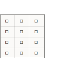
{{◻,◻,◻},
{◻,◻,◻},
{◻,◻,◻},
{◻,◻,◻}}
list of listsa table without named rows and columns 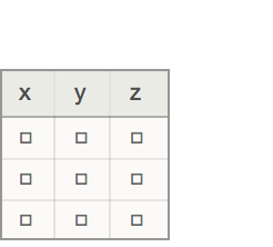
{<"x"◻,"y"◻,…>,
<"x"◻,"y"◻,…>,
<"x"◻,"y"◻,…> }
list of associationsa table with named columns 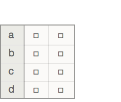
<"a"{◻,◻},
"b"{◻,◻},
"c"{◻,◻},
"d"{◻,◻}>
association of listsa table with named rows 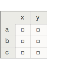
<"a"<"x"◻,"y"◻>,
"b"<"x"◻,"y"◻>,
"c"<"x"◻,"y"◻>>
association of associationsa table with named columns and named rows - Dataset interprets nested lists and associations in a row-wise fashion, so that level 1 (the outermost level) of the data is interpreted as the rows of a table, and level 2 is interpreted as the columns.
- Named rows and columns correspond to associations at level 1 and 2, respectively, whose keys are strings that contain the names. Unnamed rows and columns correspond to lists at those levels.
- Rows and columns of a dataset can be exchanged by writing Transpose[dataset].
- The following options can be given:
-
Alignment {Left,Baseline} horizontal and vertical alignments of items Background None background colors to use for items DatasetTheme Automatic overall theme for the dataset HeaderAlignment {Left,Baseline} horizontal and vertical alignments of headers HeaderBackground Automatic background colors to use for headers HeaderDisplayFunction Automatic function to use to format headers HeaderSize Automatic widths and heights of headers HeaderStyle None styles to use for headers HiddenItems None items to hide ItemDisplayFunction Automatic function to use to format items ItemSize Automatic widths and heights of items ItemStyle None styles for columns and rows MaxItems Automatic maximum number of items to display - Settings for options except HiddenItems, MaxItems and DatasetTheme can be given as follows to apply separately to different items:
-
spec apply spec to all items {speck} apply speck at successive levels {spec1,spec2,…, specn,rules} also allow explicit rules for specific parts - The speck can have the following forms:
-
{s1,s2,…,sn} use s1 through sn, then use defaults {{c}} use c in all cases {{c1,c2}} alternate between c1 and c2 {{c1,c2,…}} cycle through all ci {s,{c}} use s, then repeatedly use c {s1,{c},sn} use s1, then repeatedly use c, but use sn at the end {s1,s2,…,{c1,c2,…},sm,…,sn} use the first sequence of si at the beginning, then cyclically use the ci, then use the last sequence of si at the end {s1,s2,…,{},sm,…,sn} use the first sequence of si at the beginning and the last sequence at the end - With settings of the form {s1,s2,…,{…},sm,…,sn}, if there are more si specified than items in the dataset, si from the beginning are used for the first items, and ones from the end are used for the last items.
- Rules have the form ispec, where i specifies a position in the Dataset. Positions can be patterns.
- The position of an element can be read at the bottom of a dataset when you hover over the element.
- Settings for MaxItems can be given as follows:
-
m display m rows {m1, m2,…,mn} display mi items at dataset level i - In MaxItems, Automatic indicates that the default number of items should be displayed.
- Settings for HiddenItems can be given as follows:
-
i hide the item at position i {i1,i2,…,in} hide the items at positions ik {…, iFalse,…} show the item at position i {…, iTrue,…} hide the item at position i - Within a HiddenItems list, later settings override earlier ones.
- Individual settings for ItemDisplayFunction and HeaderDisplayFunction are pure functions that return the item to be displayed. The functions take three arguments: the item value, the item position and the dataset that contains the item.
- In some positions in ItemStyle and HeaderStyle settings, an explicit rule may be interpreted as ispec. If a style option is intended instead, wrap the rule with Directive.
- In options such as Alignment, HeaderAlignment, ItemSize and HeaderSize, which may be list-valued, a top-level list is interpreted as a single option value if possible, otherwise as a list of values for successive Dataset levels.
- If the left-hand side of a rule is not a list, the setting is applied to any position that contains the left-hand side as a key or index.
- A pure function f that returns a setting can be used in place of any setting. The setting is given by f[item,position,dataset].
- Normal can be used to convert any Dataset object to its underlying data, which is typically a combination of lists and associations.
- The syntax dataset[[parts]] or Part[dataset,parts] can be used to extract parts of a Dataset.
- The parts that can be extracted from a Dataset include all ordinary specifications for Part.
- Unlike the ordinary behavior of Part, if a specified subpart of a Dataset is not present, Missing["PartAbsent",…] will be produced in that place in the result.
- The following part operations are commonly used to extract rows from tabular datasets:
-
dataset[["name"]] extract a named row (if applicable) dataset[[{"name1",…}]] extract a set of named rows dataset[[1]] extract the first row dataset[[n]] extract the n ") row
rowdataset[[-1]] extract the last row dataset[[m;;n]] extract rows m through n dataset[[{n1,n2,…}]] extract a set of numbered rows - The following part operations are commonly used to extract columns from tabular datasets:
-
dataset[[All,"name"]] extract a named column (if applicable) dataset[[All,{"name1",…}]] extract a set of named columns dataset[[All,1]] extract the first column dataset[[All,n]] extract the n ") column
columndataset[[All,-1]] extract the last column dataset[[All,m;;n]] extract columns m through n dataset[[All,{n1,n2,…}]] extract a subset of the columns - Like Part, row and column operations can be combined. Some examples include:
-
dataset[[n,m]] take the cell at the n ") row and m
row and m") column
columndataset[[n,"colname"]] extract the value of the named column in the n ") row
rowdataset[["rowname","colname"]] take the cell at the named row and column - The following operations can be used to remove the labels from rows and columns, effectively turning associations into lists:
-
dataset[[Values]] remove labels from rows dataset[[All,Values]] remove labels from columns dataset[[Values,Values]] remove labels from rows and columns - The query syntax dataset[op1,op2,…] can be thought of as an extension of Part syntax to allow aggregations and transformations to be applied, as well as taking subsets of data.
- Some common forms of query include:
-
dataset[f] apply f to the entire table dataset[All,f] apply f to every row in the table dataset[All,All,f] apply f to every cell in the table dataset[f,n] extract the n ") column, then apply f to it
column, then apply f to itdataset[f,"name"] extract the named column, then apply f to it dataset[n,f] extract the n ") row, then apply f to it
row, then apply f to itdataset["name",f] extract the  row, then apply f to it
dataset[{nf}] selectively map f onto the n ") row
rowdataset[All,{nf}] selectively map f onto the n ") column
column - Some more specialized forms of query include:
-
dataset[Counts,"name"] give counts of different values in the named column dataset[Count[value],"name"] give number of occurences of value in the named column dataset[CountDistinct,"name"] count the number of distinct values in the named column dataset[MinMax,"name"] give minimum and maximum values in the named column dataset[Mean,"name"] give the mean value of the named column dataset[Total,"name"] give the total value of the named column dataset[Select[h]] extract those rows that satisfy condition h dataset[Select[h]/*Length] count the number of rows that satisfy condition h dataset[Select[h],"name"] select rows, then extract the named column from the result dataset[Select[h]/*f,"name"] select rows, extract the named column, then apply f to it dataset[TakeLargestBy["name",n]] give the n rows for which the named column is largest dataset[TakeLargest[n],"name"] give the n largest values in the named column - In dataset[op1,op2,…], the query operators opi are effectively applied at successively deeper levels of the data, but any given one may be applied either while "descending" into the data or while "ascending" out of it.
- The operators that make up a Dataset query fall into one of the following broad categories with distinct ascending and descending behavior:
-
All,i,i;;j,"key",… descending part operators Select[f],SortBy[f],… descending filtering operators Counts,Total,Mean,… ascending aggregation operators Query[…],… ascending subquery operators Function[…],f ascending arbitrary functions - A descending operator is applied to corresponding parts of the original dataset, before subsequent operators are applied at deeper levels.
- Descending operators have the feature that they do not change the structure of deeper levels of the data when applied at a certain level. This ensures that subsequent operators will encounter subexpressions whose structure is identical to the corresponding levels of the original dataset.
- The simplest descending operator is All, which selects all parts at a given level and therefore leaves the structure of the data at that level unchanged. All can safely be replaced with any other descending operator to yield another valid query.
- An ascending operator is applied after all subsequent ascending and descending operators have been applied to deeper levels. Whereas descending operators correspond to the levels of the original data, ascending operators correspond to the levels of the result.
- Unlike descending operators, ascending operators do not necessarily preserve the structure of the data they operate on. Unless an operator is specifically recognized to be descending, it is assumed to be ascending.
- The descending part operators specify which elements to take at a level before applying any subsequent operators to deeper levels:
-
All apply subsequent operators to each part of a list or association i;;j take parts i through j and apply subsequent operators to each part i take only part i and apply subsequent operators to it "key",Key[key] take value of key in an association and apply subsequent operators to it Values take values of an association and apply subsequent operators to each value {part1,part2,…} take given parts and apply subsequent operators to each part - The descending filtering operators specify how to rearrange or filter elements at a level before applying subsequent operators to deeper levels:
-
Select[test] take only those parts of a list or association that satisfy test SelectFirst[test] take the first part that satisfies test KeySelect[test] take those parts of an association whose keys satisfy test TakeLargestBy[f,n],TakeSmallestBy[f,n] take the n elements for which f[elem] is largest or smallest, in sorted order MaximalBy[crit],MinimalBy[crit] take the parts for which criteria crit is greater or less than all other elements SortBy[crit] sort parts in order of crit KeySortBy[crit] sort parts of an association based on their keys, in order of crit DeleteDuplicatesBy[crit] take parts that are unique according to crit DeleteMissing drop elements with head Missing - The syntax op1/*op2 can be used to combine two or more filtering operators into one operator that still operates at a single level.
- The ascending aggregation operators combine or summarize the results of applying subsequent operators to deeper levels:
-
Total total all quantities in the result Min,Max give minimum, maximum quantity in the result Mean,Median,Quantile,… give statistical summary of the result Histogram,ListPlot,… calculate a visualization on the result Merge[f] merge common keys of associations in the result using function f Catenate catenate the elements of lists or associations together Counts give association that counts occurrences of values in the result CountsBy[crit] give association that counts occurrences of values according to crit CountDistinct give number of distinct values in the result CountDistinctBy[crit] give number of distinct values in the result according to crit TakeLargest[n],TakeSmallest[n] take the largest or smallest n elements - The syntax op1/*op2 can be used to combine two or more aggregation operators into one operator that still operates at a single level.
- The ascending subquery operators perform a subquery after applying subsequent operators to deeper levels:
-
Query[…] perform a subquery on the result {op1,op2,…} apply multiple operators at once to the result, yielding a list <key1op1,key2op2,…> apply multiple operators at once to the result, yielding an association with the given keys {key1op1,key2op2,…} apply different operators to specific parts in the result - When one or more descending operators are composed with one or more ascending operators (e.g. desc/*asc), the descending part will be applied, then subsequent operators will be applied to deeper levels, and lastly, the ascending part will be applied to the result at that level.
- The special descending operator GroupBy[spec] will introduce a new association at the level at which it appears and can be inserted or removed from an existing query without affecting subsequent operators.
- Functions such as CountsBy, GroupBy, and TakeLargestBy normally take another function as one of their arguments. When working with associations in a Dataset, it is common to use this "by" function to look up the value of a column in a table.
- To facilitate this, Dataset queries allow the syntax "string" to mean Key["string"] in such contexts. For example, the query operator GroupBy["string"] is automatically rewritten to GroupBy[Key["string"]] before being executed.
- Similarly, the expression GroupBy[dataset,"string"] is rewritten as GroupBy[dataset,Key["string"]].
- Where possible, type inference is used to determine whether a query will succeed. Operations that are inferred to fail will result in a Failure object being returned without the query being performed.
- By default, if any messages are generated during a query, the query will be aborted and a Failure object containing the message will be returned.
- When a query returns structured data (e.g. a list or association, or nested combinations of these), the result will be given in the form of another Dataset object. Otherwise, the result will be given as an ordinary Wolfram Language expression.
- For more information about special behavior of Dataset queries, see the function page for Query.
- Import and SemanticImport can be used to import files as Dataset objects from formats such as "CSV" and "XLSX".
- Dataset objects can be exported with Export to formats such as "CSV", "XLSX" and "JSON".
Dataset Structure
Dataset Options
Part Operations
Dataset Queries
Descending and Ascending Query Operators
Part Operators
Filtering Operators
Aggregation Operators
Subquery Operators
Special Operators
Syntactic Shortcuts
Query Behavior
Import & Export
Examples
open all close allBasic Examples (1)
Scope (1)
Create a Dataset object from tabular data:
dataset = Dataset[{
	<|"a" -> 1, "b" -> "x", "c" -> {1}|>,
	<|"a" -> 2, "b" -> "y", "c" -> {2, 3}|>,
	<|"a" -> 3, "b" -> "z", "c" -> {3}|>,
	<|"a" -> 4, "b" -> "x", "c" -> {4, 5}|>,
	<|"a" -> 5, "b" -> "y", "c" -> {5, 6, 7}|>,
<|"a" -> 6, "b" -> "z", "c" -> {}|>}]dataset[1 ;; 3]dataset[2]A row is merely an association:
dataset[2] // NormalTake a specific element from a specific row:
dataset[3, "a"]dataset[4, "b"]dataset[5, "c"]Take the contents of a specific column:
dataset[All, "a"]dataset[All, "b"]dataset[All, "c"]Take a specific part within a column:
dataset[All, "c", 1]Take a subset of the rows and columns:
dataset[1 ;; 4, {"a", "b"}]Apply a function to the contents of a specific column:
dataset[Total, "a"]dataset[StringJoin, "b"]dataset[Catenate, "c"]Partition the dataset based on a column, applying further operators to each group:
dataset[GroupBy["b"], Catenate, "c"]dataset[All, Reverse]Apply a function both to each row and to the entire result:
dataset[Reverse, Reverse]Apply a function f to every element in every row:
dataset[All, All, f]Apply functions to each column independently:
dataset[All, {"a" -> f, "b" -> g, "c" -> h}]Construct a new table by specifying operators that will compute each column:
dataset[All, Key["c"] /* <|"ctotal" -> Total, "clength" -> Length|>]Use the same technique to rename columns:
dataset[All, <|"A" -> "a", "B" -> "b", "C" -> "c"|>]Select specific rows based on a criterion:
dataset[Select[#a < 5&]]Take the contents of a column after selecting the rows:
dataset[Select[#a < 5&], "b"]Take a subset of the available columns after selecting the rows:
dataset[Select[#a < 5&], {"b", "c"}]Take the first row satisfying a criterion:
dataset[SelectFirst[#a > 5&]]dataset[SelectFirst[#a > 5&], "b"]dataset[SortBy[Length[#c]&]]Take the rows that give the maximal value of a scoring function:
dataset[MaximalBy[Length[#c]&]]Give the top 3 rows according to a scoring function:
dataset[TakeLargestBy[Length[#c]&, 3]]Delete rows that duplicate a criterion:
dataset[DeleteDuplicatesBy["b"]]dataset[DeleteDuplicatesBy[Length[#c]&]]Compose an ascending and a descending operator to aggregate values of a column after filtering the rows:
dataset[Select[#b == "z"&] /* Total, "a"]Do the same thing by applying Total after the query:
dataset[Select[#b == "z"&], "a"][Total]Options (42)
Alignment (2)
Background (10)
Give all dataset items a pink background:
Dataset[Table[x, 4, 7], Background -> StandardPink]Dataset[Table[x, 4, 7], Background -> {{StandardPink}}]Dataset[Table[x, 4, 7], Background -> {None, {StandardPink}}]Dataset[Table[x, 4, 7], Background -> {{2, 3} -> StandardPink}]Pink and gray backgrounds for the first two rows:
Dataset[Table[x, 4, 7], Background -> {{StandardPink, StandardGray}}]Dataset[Table[x, 4, 7], Background -> {{1} -> StandardPink, {2} -> StandardGray}]Alternating pink and gray rows:
Dataset[Table[x, 4, 7], Background -> {{{StandardPink, StandardGray}}}]Alternating pink and gray columns with the first and last columns yellow:
Dataset[Table[x, 4, 7], Background -> {None, {StandardYellow, {StandardPink, StandardGray}, StandardYellow}}]Alternating pink and gray columns with the third column yellow:
Dataset[Table[x, 4, 7], Background -> {None, {{StandardPink, StandardGray}}, {All, 3} -> StandardYellow}]Dataset[Table[x, 4, 7], Background -> {{{StandardBlue, None}}, {{StandardGreen, None}}}]Set background color by value:
Dataset[IdentityMatrix[5], Background -> (If[# === 1, StandardPink, None]&)]Set background color by position:
Dataset[IdentityMatrix[5], Background -> (If[Total[#2] < 6, StandardPink, None]&)]Dataset[IdentityMatrix[5], Background -> {{2 | 4, _ ? OddQ} -> StandardPink}]DatasetTheme (4)
Use a theme with alternating row backgrounds:
Dataset[Take[ExampleData[{"Dataset", "Planets"}], All, -2], DatasetTheme -> "Detailed"]Combine themes for a customized presentation:
Dataset[EntityValue[Entity["Element", "Hydrogen"], "PropertyAssociation"], DatasetTheme -> {"Scientific", "Serif"}]Use a theme to emphasize low-level groupings:
Dataset[Nest[<|"a" -> #, "b" -> #, "c" -> #|>&, IdentityMatrix[2], 2], DatasetTheme -> "GroupDividers"]Use a theme to stripe long rows and columns to make them easier to follow:
Dataset[RandomInteger[99, {8, 12}], DatasetTheme -> {"AlternatingRowColumnBackgrounds", LightGreen, LightBlue}]HeaderAlignment (2)
HeaderBackground (2)
HeaderDisplayFunction (1)
HeaderSize (1)
HeaderStyle (4)
Set one overall style for headers:
Dataset[Take[...], HeaderStyle -> Bold]Use Directive to wrap multiple style directives:
Dataset[Take[...], HeaderStyle -> Directive[StandardBlue, FontSize -> 14]]Use a style from the current stylesheet:
Dataset[Take[...], HeaderStyle -> "Section"]Dataset[Take[...], HeaderStyle -> {{"Earth"} -> Bold, {All, "Radius"} -> StandardRed}]HiddenItems (4)
Dataset[Take[...], HiddenItems -> {3}]Dataset[Take[...], HiddenItems -> {"age"}]Hide a row except for one item:
Dataset[Take[...], HiddenItems -> {3, "age" -> False}]Hide items with a given value:
Dataset[Take[...], HiddenItems -> {"sex" -> (# === "male"&)}]ItemDisplayFunction (1)
ItemSize (3)
ItemStyle (6)
Set one overall style for dataset items:
Dataset[Table[x, 3, 5], ItemStyle -> StandardRed]Use Directive to wrap multiple style directives:
Dataset[Table[x, 3, 5], ItemStyle -> Directive[Italic, StandardBlue]]Use a style from the current stylesheet:
Dataset[Table[x, 3, 5], ItemStyle -> "Section"]Dataset[Table[x, 3, 5], ItemStyle -> {{1, 1} -> StandardRed, {2, 3} -> Underlined}]Dataset[Take[...], ItemStyle -> {"age" -> (If[# > 9, StandardRed, StandardBlue]&)}]Dataset[Table[x, 3, 5], ItemStyle -> (If[Total[#2] < 5, StandardRed, StandardBlue]&)]Applications (3)
Tables (Lists of Associations) (1)
Load a dataset of passengers of the Titanic:
titanic = ExampleData[{"Dataset", "Titanic"}]Length[titanic]Get a random sample of passengers:
RandomSample[titanic, 5]The underlying data is a list of associations:
Normal[%]Count the number of passengers with a missing age:
titanic[Count[_Missing], "age"]Count the number of passengers in 1st, 2nd and 3rd class:
titanic[Counts, "class"]Get a histogram of passenger ages:
titanic[Histogram, "age"]Get a histogram of passenger ages, grouped by passenger class:
titanic[GroupBy["class"], Histogram[#, {0, 80, 4}]&, "age"]Find the age of the oldest passenger:
titanic[Max, "age"]Calculate the overall survival ratio:
ratio[list_] := list // Boole//Mean//N;titanic[ratio, "survived"]Show the survival ratio against sex and passenger class:
titanic[GroupBy["sex"], GroupBy["class"], ratio, "survived"]Show the survival ratio as a function of age:
titanic[GroupBy[Round[#age, 5]&], ratio, "survived"]//ListPlotIndexed Tables (Associations of Associations) (1)
Load a dataset of planets and their properties:
planets = ExampleData[{"Dataset", "Planets"}]Look up the mass of the Earth:
planets["Earth", "Mass"]Get the subtable corresponding to moons of a specific planet:
planets["Neptune", "Moons"]Produce a dataset of the radii of the planets:
planets[All, "Radius"]Visualize the radii of the planets:
planets[BarChart, "Radius"]Produce a dataset of the number of moons of each planet:
planets[All, "Moons", Length]PieChart[%, ChartLegends -> Automatic]Obtain a list of the planets and their masses, sorted by increasing mass:
planets[SortBy["Mass"], "Mass"]Find the total mass of each planet's moons:
planets[All, "Moons", Total, "Mass"]Obtain a list of only those moons that have a mass larger than half that of Earth's moon:
moonMass = planets["Earth", "Moons", "Moon", "Mass"];
planets[All, "Moons", Select[#Mass > moonMass / 2&] /* Keys]
Find the heaviest moon of each planet:
planets[All, "Moons", MaximalBy["Mass"] /* Keys]Obtain a list of all planetary moons:
moons = planets[Catenate, "Moons"]Make a scatter plot of the mass against radius:
moons[ListLogLogPlot, {#Mass, #Radius}&]Calculate and make a histogram of the densities:
sphereVolume = [image];
moons[Histogram, #Mass  / sphereVolume[#Radius]&]
Compute the mean density for the moons of each planet:
planets[All, "Moons", Mean, #Mass / sphereVolume[#Radius]&]Create a table comparing the density of each planet with the mean density of its moons:
density = #Mass / sphereVolume[#Radius]&;planets[All, <|"Planet Density" -> density, "Moon Density" -> Query["Moons", Mean, density]|>]Hierarchical Data (Associations of Associations of Other Data) (1)
Load a dataset associating countries to their administrative divisions to their populations:
populations = ExampleData[{"Dataset", "StatePopulations"}]The underlying data is an association whose keys are countries and whose values are further associations between administrative divisions and their populations:
Normal @ populations[1 ;; 2, 1 ;; 2]Look up the populations for a specific country:
populations[["south africa"]]Give the total population (not all countries in the world are included in this dataset):
populations[Total, Total]Count the number of divisions within each country:
populations[All, Length]Total the number of divisions:
populations[Total, Length]Build a histogram of the number of divisions:
populations[Histogram, Length]Calculate the total population of each country by adding the populations of each division:
populations[All, Total]Obtain the five most populous countries:
populations[All, Total][Sort][-5 ;; -1]Obtain the most populous divisions for each country:
populations[All, MaximalBy[Total] /* Keys /* First]Correlate the number of divisions a country has with its population:
populations[ListLogPlot, {Length, Total}]The underlying data being passed to ListLogPlot is an association of lists, each of length 2:
populations[1 ;; 5, {Length, Total}]Normal[%]Properties & Relations (4)
Query is the operator form of the query language supported by Dataset:
Query["b", Total] @ <|"a" -> {1, 2}, "b" -> {3, 4}|>Dataset[<|"a" -> {1, 2}, "b" -> {3, 4}|>]["b", Total]Use EntityValue to obtain a Dataset of the properties of Entity objects from the Wolfram Knowledgebase:
gases = EntityValue[["noble gasses"], {"BoilingPoint", "Density"}, "Dataset"]Plot the boiling point versus density on a log plot:
ListLogPlot[gases]Use SemanticImport to import a file as a Dataset:
sales = SemanticImport["ExampleData/RetailSales.tsv"]Calculate the total quantity of sales:
sales[Total, "Sales"]Obtain a small sample of the Titanic passenger dataset:
sample = RandomSample[ExampleData[{"Dataset", "Titanic"}], 5]Export the sample as "JSON" format:
ExportString[sample, "JSON"]Data with named columns can be more compactly represented if it is first transposed:
ExportString[Transpose @ sample, "JSON"]Export the sample as "CSV":
ExportString[sample, "CSV"]Possible Issues (3)
Data without a consistent structure will not usually format in the same way as structured data:
Dataset[{<|"A" -> 1, "B" -> 2|>, <|"A" -> 3, "B" -> 4|>, <|"A" -> 5, "B" -> 6|>}]Dataset[{<|"A" -> 1, "B" -> 2|>, <|"A" -> 3, "B" -> 4|>, {5, 6}}]If a sub-operation of a query is inferred to fail, the entire query will not be performed, and a Failure object will be returned:
Dataset[<|"A" -> 1, "B" -> 2|>]["C"]By default, if any messages are generated during an operation on a Dataset, a Failure object will be returned:
Dataset[{"abc", "abdefg", "ab"}][All, StringTake[#, 3]&]To specify different behavior, use an explicit Query expression in conjunction with the option FailureAction:
Query[All, StringTake[#, 3]&, FailureAction -> "Replace"] @ Dataset[{"abc", "abdefg", "ab"}]Neat Examples (2)
Calculate the survival likelihood of the characters Jack Dawson and Rose DeWitt Bukater from the movie Titanic by matching them with real passengers:
titanic = ExampleData[{"Dataset", "Titanic"}];characters = <|
"Rose" -> <|"class" -> "1st", "age" -> 17, "sex" -> "female"|>,
"Jack" -> <|"class" -> "3rd", "age" -> 20, "sex" -> "male"|>
|>;matches[target_][passenger_] := target == KeyDrop[passenger, "survived"];titanic[Select[matches[#]], "survived"]& /@ charactersMap[Normal /* Boole /* Mean, %]Make an interactive control that plots a heat map of a country's divisions when a country is selected:
populations = ExampleData[{"Dataset", "StatePopulations"}];populations[KeyTake[{Entity["Country", "Brazil"], Entity["Country", "China"], Entity["Country", "India"]}]][TabView, GeoRegionValuePlot[#, ImageSize -> Medium, GeoBackground -> None]&]Related Links
Text
Wolfram Research (2014), Dataset, Wolfram Language function, https://reference.wolfram.com/language/ref/Dataset.html (updated 2021).
CMS
Wolfram Language. 2014. "Dataset." Wolfram Language & System Documentation Center. Wolfram Research. Last Modified 2021. https://reference.wolfram.com/language/ref/Dataset.html.
APA
Wolfram Language. (2014). Dataset. Wolfram Language & System Documentation Center. Retrieved from https://reference.wolfram.com/language/ref/Dataset.html