MagneticPDEComponent
MagneticPDEComponent[vars,pars]
yields a magnetic PDE term with variables vars and pars.
Details
- MagneticPDEComponent generates an equation to model magnetostatics and low-frequency electromagnetics with model variables vars and model parameters pars.
- MagneticPDEComponent returns a sum of differential operators to be used as a part of partial differential equations:
- MagneticPDEComponent models static magnetic fields produced by permanent magnets or magnetic and electric fields that are generated by low-frequency electric currents flowing in conductive materials.
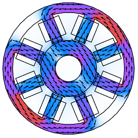
- MagneticPDEComponent is typically used to model electric motors, inductors and electromagnets.
- MagneticPDEComponent creates PDE components for stationary, time, frequency and parametric analysis.
- MagneticPDEComponent models magnetostatics and low-frequency electromagnetic phenomena with the dependent magnetic vector potential
 in units of [
![TemplateBox[{InterpretationBox[, 1], {"Wb", , "/", , "m"}, webers per meter, {{(, "Webers", )}, /, {(, "Meters", )}}}, QuantityTF] TemplateBox[{InterpretationBox[, 1], {"Wb", , "/", , "m"}, webers per meter, {{(, "Webers", )}, /, {(, "Meters", )}}}, QuantityTF]](Files/MagneticPDEComponent.en/4.png) ] and independent variables
] and independent variables  in units of [
![TemplateBox[{InterpretationBox[, 1], "m", meters, "Meters"}, QuantityTF] TemplateBox[{InterpretationBox[, 1], "m", meters, "Meters"}, QuantityTF]](Files/MagneticPDEComponent.en/6.png) ].
]. - MagneticPDEComponent can model external currents also in the static case.
- In the static case, when no currents are present, MagnetostaticPDEComponent should be used.
- The vector-valued dependent variable
 is specified as a three-vector
  ={Ax1,Ax2,Ax3}.
 - Stationary variables vars are vars={
 [x1,…,xn],{x1,…,xn}}.
 - Frequency-dependent variables vars are vars={
 [x1,…,xn],ω,{,…,xn}}.
 - Time-dependent variables vars are vars={
 [t,x1,…,xn],t,{x1,…,xn}}.
 - MagneticPDEComponent provides a stationary magnetic model:
 is the vacuum permeability in units of [
![TemplateBox[{InterpretationBox[, 1], {"H", , "/", , "m"}, henries per meter, {{(, "Henries", )}, /, {(, "Meters", )}}}, QuantityTF] TemplateBox[{InterpretationBox[, 1], {"H", , "/", , "m"}, henries per meter, {{(, "Henries", )}, /, {(, "Meters", )}}}, QuantityTF]](Files/MagneticPDEComponent.en/14.png) ],
],  the magnetization vector in units of [
![TemplateBox[{InterpretationBox[, 1], {"A", , "/", , "m"}, amperes per meter, {{(, "Amperes", )}, /, {(, "Meters", )}}}, QuantityTF] TemplateBox[{InterpretationBox[, 1], {"A", , "/", , "m"}, amperes per meter, {{(, "Amperes", )}, /, {(, "Meters", )}}}, QuantityTF]](Files/MagneticPDEComponent.en/16.png) ] and
] and  the external current density vector in units of [
![TemplateBox[{InterpretationBox[, 1], {"A", , "/", , {"m", ^, 2}}, amperes per meter squared, {{(, "Amperes", )}, /, {(, {"Meters", ^, 2}, )}}}, QuantityTF] TemplateBox[{InterpretationBox[, 1], {"A", , "/", , {"m", ^, 2}}, amperes per meter squared, {{(, "Amperes", )}, /, {(, {"Meters", ^, 2}, )}}}, QuantityTF]](Files/MagneticPDEComponent.en/18.png) ].
].- The magnetization vector
 specifies the magnetic dipole moment per unit volume within a material, indicating the strength and direction of its magnetic properties.
 - MagneticPDEComponent provides a frequency domain model:
 [
[![TemplateBox[{InterpretationBox[, 1], {"F", , "/", , "m"}, farads per meter, {{(, "Farads", )}, /, {(, "Meters", )}}}, QuantityTF] TemplateBox[{InterpretationBox[, 1], {"F", , "/", , "m"}, farads per meter, {{(, "Farads", )}, /, {(, "Meters", )}}}, QuantityTF]](Files/MagneticPDEComponent.en/22.png) ] is the vacuum permittivity, relative permittivity
] is the vacuum permittivity, relative permittivity  [-], electrical conductivity
  [
[![TemplateBox[{InterpretationBox[, 1], {"S", , "/", , "m"}, siemens per meter, {{(, "Siemens", )}, /, {(, "Meters", )}}}, QuantityTF] TemplateBox[{InterpretationBox[, 1], {"S", , "/", , "m"}, siemens per meter, {{(, "Siemens", )}, /, {(, "Meters", )}}}, QuantityTF]](Files/MagneticPDEComponent.en/25.png) ], angular frequency
], angular frequency  [
[![TemplateBox[{InterpretationBox[, 1], {"rad", , "/", , "s"}, radians per second, {{(, "Radians", )}, /, {(, "Seconds", )}}}, QuantityTF] TemplateBox[{InterpretationBox[, 1], {"rad", , "/", , "s"}, radians per second, {{(, "Radians", )}, /, {(, "Seconds", )}}}, QuantityTF]](Files/MagneticPDEComponent.en/27.png) ] and the imaginary unit
] and the imaginary unit  .
.- MagneticPDEComponent provides a time domain model:
- An alternative model to the magnetization vector
 , is the remanent magnetic flux density vector
  in units of [
![TemplateBox[{InterpretationBox[, 1], {"Wb", , "/", , {"m", ^, 2}}, webers per meter squared, {{(, "Webers", )}, /, {(, {"Meters", ^, 2}, )}}}, QuantityTF] TemplateBox[{InterpretationBox[, 1], {"Wb", , "/", , {"m", ^, 2}}, webers per meter squared, {{(, "Webers", )}, /, {(, {"Meters", ^, 2}, )}}}, QuantityTF]](Files/MagneticPDEComponent.en/32.png) ].
]. - The stationary MagneticPDEComponent equation is given as:
 is the unitless recoil permeability.
- For linear materials, the stationary equation MagneticPDEComponent simplifies to:
 is the unitless relative permeability.
 can be isotropic, orthotropic or anisotropic.
 can be a function of the magnetic field and describe nonlinear materials.
- The units of the magnetic model terms are in [
![TemplateBox[{InterpretationBox[, 1], {"A", , "/", , {"m", ^, 2}}, amperes per meter squared, {{(, "Amperes", )}, /, {(, {"Meters", ^, 2}, )}}}, QuantityTF] TemplateBox[{InterpretationBox[, 1], {"A", , "/", , {"m", ^, 2}}, amperes per meter squared, {{(, "Amperes", )}, /, {(, {"Meters", ^, 2}, )}}}, QuantityTF]](Files/MagneticPDEComponent.en/39.png) ].
]. - The following parameters pars can be given:
-
parameter default symbol "ExternalCurrentSource" {0,…}  , external current density vector in [
![TemplateBox[{InterpretationBox[, 1], {"A", , "/", , {"m", ^, 2}}, amperes per meter squared, {{(, "Amperes", )}, /, {(, {"Meters", ^, 2}, )}}}, QuantityTF] TemplateBox[{InterpretationBox[, 1], {"A", , "/", , {"m", ^, 2}}, amperes per meter squared, {{(, "Amperes", )}, /, {(, {"Meters", ^, 2}, )}}}, QuantityTF]](Files/MagneticPDEComponent.en/41.png) ]
]"Magnetization" {0,…}  , magnetization vector in [
![TemplateBox[{InterpretationBox[, 1], {"A", , "/", , "m"}, amperes per meter, {{(, "Amperes", )}, /, {(, "Meters", )}}}, QuantityTF] TemplateBox[{InterpretationBox[, 1], {"A", , "/", , "m"}, amperes per meter, {{(, "Amperes", )}, /, {(, "Meters", )}}}, QuantityTF]](Files/MagneticPDEComponent.en/43.png) ]
]"MagneticModelForm" None 
"RegionSymmetry" None 
"RelativePermeability"  , unitless relative permeability
"RemanentMagneticFluxDensity" {0,…}  , remanent magnetic flux density in [
![TemplateBox[{InterpretationBox[, 1], {"Wb", , "/", , {"m", ^, 2}}, webers per meter squared, {{(, "Webers", )}, /, {(, {"Meters", ^, 2}, )}}}, QuantityTF] TemplateBox[{InterpretationBox[, 1], {"Wb", , "/", , {"m", ^, 2}}, webers per meter squared, {{(, "Webers", )}, /, {(, {"Meters", ^, 2}, )}}}, QuantityTF]](Files/MagneticPDEComponent.en/48.png) ]
]"Thickness" 1  , thickness in [
![TemplateBox[{InterpretationBox[, 1], "m", meters, "Meters"}, QuantityTF] TemplateBox[{InterpretationBox[, 1], "m", meters, "Meters"}, QuantityTF]](Files/MagneticPDEComponent.en/50.png) ]
] "VacuumPermeability" 
 , vacuum permeability in [
![TemplateBox[{InterpretationBox[, 1], {"H", , "/", , "m"}, henries per meter, {{(, "Henries", )}, /, {(, "Meters", )}}}, QuantityTF] TemplateBox[{InterpretationBox[, 1], {"H", , "/", , "m"}, henries per meter, {{(, "Henries", )}, /, {(, "Meters", )}}}, QuantityTF]](Files/MagneticPDEComponent.en/53.png) ]
] - Additional parameters can be specified for the frequency and time domain models:
-
parameter default symbol "ElectricalConductivity" 1  , electrical conductivity in [
![TemplateBox[{InterpretationBox[, 1], {"S", , "/", , "m"}, siemens per meter, {{(, "Siemens", )}, /, {(, "Meters", )}}}, QuantityTF] TemplateBox[{InterpretationBox[, 1], {"S", , "/", , "m"}, siemens per meter, {{(, "Siemens", )}, /, {(, "Meters", )}}}, QuantityTF]](Files/MagneticPDEComponent.en/55.png) ]
]
- The number of independent variables
 determines the dimensions of
  ,
,  and
and  and the length of vectors
  ,
,  and
and  .
. - The models are available in a 2D, a 2D axisymmetric and a 3D form.
- For 3D stationary models with relative permeability
 , "MagneticModelForm" can be set to "FreeSpace", and with the Coulomb gauge condition,
  , the 3D operator simplifies to:
 - In 2D, with an out-of-plane direction, the magnetic vector potential has only a
 component. In the stationary linear case, the equation is given by:
  [
[![TemplateBox[{InterpretationBox[, 1], "m", meters, "Meters"}, QuantityTF] TemplateBox[{InterpretationBox[, 1], "m", meters, "Meters"}, QuantityTF]](Files/MagneticPDEComponent.en/69.png) ] is a variable denoting a "Thickness" in the
] is a variable denoting a "Thickness" in the  direction and the dependent variable
  is specified as
  ={0,0,Az}.
- A possible choice for the parameter "RegionSymmetry" is "Axisymmetric".
- "Axisymmetric" region symmetry represents a truncated cylindrical coordinate system where the cylindrical coordinates are reduced by removing the angle variable as follows:
-
dimension reduction e.g. linear stationary equation 2D 

- To solve this equation, the covariant formulation is made use of. The covariant formulation is a method in which a change of variable is applied to axisymmetric equation, given by
 :
: - The input specification for the parameters is exactly the same as for their corresponding operator terms.
- If no parameters are specified, the default magnetic PDE is:
- If the MagneticPDEComponent depends on parameters
 that are specified in the association pars as …,keypi…,pivi,…], the parameters
  are replaced with
  .
.
Examples
open allclose allBasic Examples (3)
Scope (7)
Define a magnetic PDE model with a relative permeability set to 5:
Activate a magnetic PDE model:
Define a symbolic 2D out-of-plane magnetic PDE model with vacuum permeability ![]() , relative permeability
, relative permeability ![]() and an external current in the
and an external current in the ![]() direction:
direction:
Note that the ![]() and
and ![]() direction currents are not considered:
direction currents are not considered:
Define a symbolic 2D axisymmetric magnetic PDE model:
Note that the ![]() and
and ![]() direction currents are not considered:
direction currents are not considered:
Define a 3D free-space magnetic PDE model with relative permeability of 1:
Define a symbolic 2D-frequency magnetic PDE model:
Set up the default magnetic PDE model with vacuum permeability ![]() and relative permeability
and relative permeability ![]() and maintain Quantity objects:
and maintain Quantity objects:
Applications (2)
2D Stationary Analysis (1)
2D Frequency Analysis (1)
Define the mesh to model a long copper wire of circular cross section:
Define the parameters of the model with:
Define the uniform external current density in the ![]() direction:
direction:
Define a zero magnetic potential condition at the exterior boundary:
Set up an angular frequency of 800 Hz:
Replace the angular frequency ![]() and solve the PDE:
and solve the PDE:
Text
Wolfram Research (2025), MagneticPDEComponent, Wolfram Language function, https://reference.wolfram.com/language/ref/MagneticPDEComponent.html.
CMS
Wolfram Language. 2025. "MagneticPDEComponent." Wolfram Language & System Documentation Center. Wolfram Research. https://reference.wolfram.com/language/ref/MagneticPDEComponent.html.
APA
Wolfram Language. (2025). MagneticPDEComponent. Wolfram Language & System Documentation Center. Retrieved from https://reference.wolfram.com/language/ref/MagneticPDEComponent.html