Electromagnetism
| Contents | Skin Depth |
| Introduction | Frequency versus Time Domain |
| Maxwell's Equations | Phasors |
| Constitutive Relations | Nomenclature |
| Types of Electromagnetics Modeling | References |
Contents
Introduction
In this monograph, an overview of electromagnetism is given. Electromagnetism, from an engineering perspective, is the analysis and study of devices involving electric, magnetic or electromagnetic (EM) phenomena. These devices come from seemingly diverse areas such as electric machines, capacitors or waveguides and antennas. Even though each of the devices mentioned can have different characteristics, all can fundamentally be described by Maxwell's equations. As the Maxwell equations are fundamental to describing the behavior of electric and magnetic fields in space, the equations form the basic building blocks for modeling EM devices.
In many applications, one is unlikely to consider the whole formulation of electromagnetism. Instead, subfields of electromagnetism are used, in which assumptions are taken, leading to simplifications of Maxwell's equations, such as in electrostatics or magnetostatics. These simplified equations are usually based on a vector field, a potential or both.
This notebook will provide an overview of the theory of electromagnetics, so at the end the reader has an understanding of the fundamentals and formulations used. Depending on if one wants to solve for a steady-state electric field or magnetic field, a time-varying magnetic or electric field or the whole EM field, one needs to choose a specific governing equation. A key learning element of this notebook is how to dispatch various applications to the respective subfields.
Once there is an understanding of how to model a specific device, the following listed monographs are more specialized. They explain theory, equations and boundary conditions specific to electromagnetic analysis in greater detail than presented here. Each monograph provides overview examples relevant to its respective topic.
The areas covered will be expanded upon in future versions of the Wolfram Language. The first two monographs focuses on stationary fields, while the rest focus on transient fields.
The following sections of this notebook focus on the general background that these subcases of electromagnetics have in common, such as the Maxwell's equations, the constitutive relations, potentials, phasors and boundary conditions.
The key point of this overview is to provide guidance on finding the best modeling approach for a specific application, and the details will be discussed in the Types of Electromagnetics Modeling section.
Maxwell's Equations
The partial differential equations to be solved are Maxwell's equations, a set of partial differential equations in time and space that describe the relationship between the electric and magnetic fields and their sources. The equations describe the behavior of the fields in the presence of charges and currents, and they can be written in short form using differential vector operators.
Maxwell's equations are given by:
where ![]() is the gradient operator,
is the gradient operator, ![]() is the dot product and
is the dot product and ![]() is the cross product. All vector-valued quantities are bold.
is the cross product. All vector-valued quantities are bold. ![]() [
[![]() ] and
] and ![]() [
[![]() ] are the electric and magnetic fields' intensity, respectively.
] are the electric and magnetic fields' intensity, respectively. ![]() [
[![]() ] is the electric flux density, and
] is the electric flux density, and ![]() [
[![]() ]
]![]() [
[![]() ] is the magnetic flux density, sometimes also called magnetic induction. A flux density refers to a flow though an area.
] is the magnetic flux density, sometimes also called magnetic induction. A flux density refers to a flow though an area. ![]() [
[![]() ] is electric charge density and
] is electric charge density and ![]() [
[![]() ] is the electric current flux density, commonly called electric current density, and they represent sources of electric and magnetic fields, respectively. SI units are used throughout all electromagnetics monographs.
] is the electric current flux density, commonly called electric current density, and they represent sources of electric and magnetic fields, respectively. SI units are used throughout all electromagnetics monographs.
In this monograph, when the terms electric or magnetic fields are used without explicitly specifying the symbol name, they generically refer to either of the fields, such as ![]() or
or ![]() and
and ![]() or
or![]() . In these cases, the specific field being referenced is not critical.
. In these cases, the specific field being referenced is not critical.
Another fundamental equation, known as the equation of continuity, is
To make these equations solvable, constitutive relations must be defined, such as Ohm's law, which specifies how electromagnetic fields interact with media.
Constitutive Relations
Constitutive relations are relations between physical quantities specific to a material and describe a medium's macroscopic properties. In other words, specifying material properties establishes the relationship of the field vectors ![]() and
and ![]() to
to ![]() ,
, ![]() , and
, and ![]() .
.
The first constitutive relation is given by:
where ![]() is the permittivity of vacuum [
is the permittivity of vacuum [![]() ], and the second term
], and the second term ![]() [
[![]() ] is the polarization vector.
] is the polarization vector.
The second constitutive relation is:
where ![]() is the permeability of vacuum [
is the permeability of vacuum [![]() ], and
], and ![]() [
[![]() ] is the magnetization vector.
] is the magnetization vector.
Alternatively, a magnetic polarization ![]() [
[![]() ]
]![]() [
[![]() ] can be defined, such that
] can be defined, such that ![]() . The relation between the magnetic polarization and the magnetization vector is then given by
. The relation between the magnetic polarization and the magnetization vector is then given by ![]() .
.
In either case, materials can have a nonzero ![]() or
or ![]() even when there is no electric or magnetic field, respectively. A permanent magnet would be a case where there is a nonzero
even when there is no electric or magnetic field, respectively. A permanent magnet would be a case where there is a nonzero ![]() .
.
Finally, the last constitutive relation is between the electric field ![]() and the current density
and the current density ![]() , given by Ohm's law:
, given by Ohm's law:
where ![]() is the electrical conductivity [
is the electrical conductivity [![]() ] of the medium.
] of the medium.
Linear Constitutive Relations
For the special but important case of linear materials, the polarization ![]() and magnetization
and magnetization ![]() vectors are directly proportional to magnetic and electric field intensity. Their relations can be stated as:
vectors are directly proportional to magnetic and electric field intensity. Their relations can be stated as:
where the unitless factors ![]() and
and ![]() are the electric and the magnetic susceptibility. For such linear materials, the constitutive relations are obtained by reinserting Eqns. 1 and 2 into 3 and 4:
are the electric and the magnetic susceptibility. For such linear materials, the constitutive relations are obtained by reinserting Eqns. 1 and 2 into 3 and 4:
where the unitless ![]() and
and ![]() [
[![]() ] are the relative and absolute permittivity, respectively, and the unitless
] are the relative and absolute permittivity, respectively, and the unitless ![]() and
and ![]() [
[![]() ] are the relative and absolute permeability.
] are the relative and absolute permeability.
In general, ![]() and
and ![]() are tensors that depend on spatial or other variables; for several materials, good simplified approximations are available, but that depends on the material at hand. Some special cases are listed below:
are tensors that depend on spatial or other variables; for several materials, good simplified approximations are available, but that depends on the material at hand. Some special cases are listed below:
In the most general case, constitutive relations are nonlinear; that is, the permeability, the conductivity and the permittivity depend on the field with which they are associated:
Constitutive Relations Summary
The following table summarizes the main quantities and the constitutive relations used for describing EM fields.
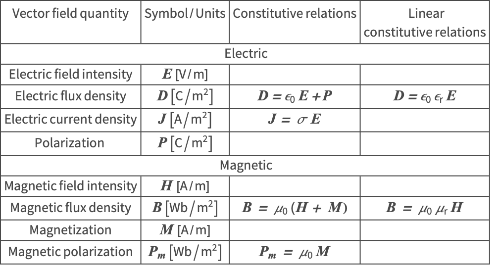
Table specifying the vector field quantities in electromagnetism and its constitutive relations.
Types of Electromagnetics Modeling
Solving the full Maxwell's equations is typically computationally intensive in terms of CPU and computer memory usage. Therefore, it is common practice to make reasonable assumptions that lead to simplified equations, enabling a more efficient solution process. The goal of this notebook is to present these simplified equations and provide guidance on when to use each type. These simplified equations often rely on vector fields, potentials or both.
Dependent Variables
Under certain circumstances, Maxwell's equations can be simplified and reformulated in terms of the scalar electric potential ![]() [
[![]() ], the magnetic vector potential
], the magnetic vector potential ![]() [
[![]() ] or the magnetic scalar potential
] or the magnetic scalar potential ![]() [
[![]() ].
].
The electric scalar potential ![]() is related to the electric field intensity by the following equation:
is related to the electric field intensity by the following equation:
The negative sign was placed by convenience and for historical reasons.
If one wanted to use the same scalar electric potential shown in (5) to represent a time-dependent electric field, an additional term would have to be added:
A relation between the magnetic potential vector ![]() and the magnetic flux density
and the magnetic flux density ![]() is given by the following equation:
is given by the following equation:
Last, when there are no free currents, ![]() and under static conditions, it is also possible to define a magnetic scalar potential
and under static conditions, it is also possible to define a magnetic scalar potential ![]() , similar to the scalar electric potential
, similar to the scalar electric potential ![]() . The scalar magnetic potential
. The scalar magnetic potential ![]() can be defined as:
can be defined as:
The actual derivation of these relations is presented in the Electrostatics, Electric Currents and the Magnetostatics for Permanent Magnets monographs. For now it is only important to know that they exist.
Electromagnetics Decision Diagram
Next, a rule of thumb is provided regarding which equations and functions to use in different modeling scenarios. The following flow chart assists in deciding the approach for an electromagnetics simulation and will be explained in the subsequent text.

The figure presents a flow chart that gives a rule of thumb on which functions to use in which electromagnetics modeling scenario.
The first question to ask is whether the planned simulation is static or transient. If neither the electric nor the magnetic field varies over time due to the absence of time-varying inputs, then it can be assumed that the case is static.
Statics
In this regime, steady-state fields produced by direct currents (DC), static charges or magnetic domains are assumed. The main assumption here is that fields do not vary in time. This means that ![]() and
and ![]() . As a consequence, in the static case, the electric and magnetic fields are no longer coupled. Faraday's law (Eqn. 6) is no longer coupled to
. As a consequence, in the static case, the electric and magnetic fields are no longer coupled. Faraday's law (Eqn. 6) is no longer coupled to ![]()
and Ampere's law (Eqn. 7) is no longer coupled to ![]()
Therefore, one can solve for ![]() independently of
independently of ![]() and vice versa. The next question is, Which of the fields is of interest?
and vice versa. The next question is, Which of the fields is of interest?
Electric field
Depending on the constitutive relations of interest, one chooses from:
- Electrostatics: Describes electric fields generated by nonmoving, static charges. Used to model insulating or dielectric materials. In this case, the scalar electric potential
 is solved for, and subsequently for the electric field intensity
  . The electrostatic equation is given by:
The concepts of electrostatics simulations are discussed in the Electrostatics monograph, and ElectrostaticPDEComponent is the function that yields an electrostatic PDE term.
- Stationary currents: Describe the steady current flow in conductive materials such as metals. In this case, the scalar electric potential
 is solved for, and subsequently the current density
  and electric field intensity
  . The electric current equation is given by:
The concepts of stationary currents simulations are discussed in the Electric Currents monograph, and ElectricCurrentPDEComponent is the function that yields a stationary electric current PDE term.
When direct currents (DC) are simulated, magnetic fields are produced as a byproduct. However, since the magnetic field is stationary, it does not generate induced currents. As a result, once the steady currents are known, the magnetic field is fully determined and can be computed in a subsequent step by using ![]() , which is solved in the magnetostatics case.
, which is solved in the magnetostatics case.
Magnetic field
- Magnetostatics: describes magnetic fields produced either by permanent magnets or by direct currents (DC). In this case, the magnetic scalar potential
 or the magnetic vector potential
  is solved for, and subsequently the magnetic flux density
 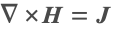 . The
. The  formulation can handle currents, while the scalar formulation based on
  cannot.
The scalar magnetic potential equation is given by:
The concepts of scalar magnetostatics simulations are discussed in the Magnetostatics for Permanent Magnets monograph, and MagnetostaticPDEComponent is the function that yields a stationary magnetic PDE term.
The magnetic vector potential is given by:
Transient
If fields vary in time, a time-dependent analysis is necessary. Initially, it is important to determine whether the model belongs in the low- or high-frequency regime to establish whether the magnetic and electric fields can be modeled using quasistatic approximations or the fields should be treated as electromagnetic waves.
Transient equations can typically be formulated in what is called the frequency domain or the time domain. The frequency domain is generally preferable when applicable, since it allows for faster simulations. Do not confuse the frequency domain with the frequency regime. The frequency regime classifies if a device is operated in a low- or high-frequency regime, while the frequency domain is a simulation technique that allows for efficient simulations.
Frequency regime
At low frequency, electromagnetic radiation is negligible [Humphries, 2010]. This means that the electric and magnetic fields are not fully coupled, so some time-derivative terms can be neglected, simplifying the equations. This scenario is called quasistatic.
The quasistatic approximations are based on having sufficiently slow time variations and sufficiently small dimensions so that the time required for an electromagnetic wave to propagate at the velocity ![]() over the object size
over the object size ![]() is short compared to the total simulation time of interest
is short compared to the total simulation time of interest ![]() :
:
where the ratio ![]() is the time required for an electromagnetic wave to propagate through a length
is the time required for an electromagnetic wave to propagate through a length ![]() .
.
Eqn. 8 can be reformulated in terms of the wavelength ![]() . In this case, electromagnetic radiation is negligible if the wavelength
. In this case, electromagnetic radiation is negligible if the wavelength ![]() is much larger than the object size
is much larger than the object size ![]() :
:
The wavelength is given by ![]() , where
, where ![]() is the phase speed of the wave in [
is the phase speed of the wave in [![]() ] and
] and ![]() the wave's frequency in [
the wave's frequency in [![]() ], related to the angular frequency by
], related to the angular frequency by ![]() . As a rule of thumb: if the wavelength of the electromagnetic wave is much larger than the characteristic size of the object,
. As a rule of thumb: if the wavelength of the electromagnetic wave is much larger than the characteristic size of the object, ![]() , then it can be assumed that the system is in a low-frequency regime.
, then it can be assumed that the system is in a low-frequency regime.
If the characteristic size of the object ![]() approaches a fraction of the wavelength, say,
approaches a fraction of the wavelength, say, ![]() , then the system is in the high-frequency regime, requiring the use of an electromagnetic wave equation.
, then the system is in the high-frequency regime, requiring the use of an electromagnetic wave equation.
Next, the low-frequency regime and the high-frequency regime will be described in more detail.
Low-frequency regime—Quasistatic
In a low-frequency scenario, it is necessary to determine whether it is sufficient to consider only the electric field or if both electric and magnetic fields need to be considered. To do this, compute the skin depth ![]() [
[![]() ] of the device and compare it to the device's characteristic size
] of the device and compare it to the device's characteristic size ![]() [
[![]() ].
].
When the skin depth of the material is much larger than the characteristic size of the device, ![]() magnetic effects can be ignored. Since the skin effect is negligible, inductive effects can be neglected, one need not consider the magnetic flux density
magnetic effects can be ignored. Since the skin effect is negligible, inductive effects can be neglected, one need not consider the magnetic flux density ![]() and can use the following equation:
and can use the following equation:
It can be shown that this formulation allows the electroquasistatics approximation with electric potential ![]() to be used. To be clear,
to be used. To be clear, ![]() and
and ![]() , but in this approach they are ignored because the inductive effects are negligible. That is why in the above equation the approximate sign
, but in this approach they are ignored because the inductive effects are negligible. That is why in the above equation the approximate sign ![]() is used.
is used.
- Electroquasistatics—Frequency domain: Describes harmonic electric fields generated by alternating currents, which are composed of a conduction current
 and a displacement current
  . In this approximation, the scalar electric potential
  is solved for, and subsequently the electric field intensity
  .
.
- Electroquasistatics—Time domain: Describes time-varying electric fields generated by time-varying currents, which are composed of a conduction current and a displacement current
 . In this approximation, the scalar electric potential
  is solved for, and subsequently the electric field intensity
  .
.
The concepts of electroquasistatic simulations are discussed in more depth in the Electric Currents monograph, and ElectricCurrentPDEComponent is the function that yields both a frequency-domain and a time-domain electric current PDE term.
When the skin depth of the material is much smaller than the characteristic size of the device, ![]() , or if the magnetic field is of primary interest, or if there are electric fields that produce inductive effects, a magnetoquasistatic analysis needs to be performed.
, or if the magnetic field is of primary interest, or if there are electric fields that produce inductive effects, a magnetoquasistatic analysis needs to be performed.
Alternating currents in a conductor produce a magnetic field as a side product. This magnetic field will induce secondary currents, known as Eddy currents and a secondary electric field. These are non-negligible inductive effects, and the magnetoquasistatic analysis takes care of them.
If the skin depth is equal to or smaller than the characteristic size ![]() ,
, ![]() , then these inductive effects are important and both electric and magnetic fields need to be considered.
, then these inductive effects are important and both electric and magnetic fields need to be considered.
In this case, the following equation is used:
- Magnetoquasistatics—Frequency domain: Describes harmonic magnetic fields in the low-frequency regime. In the case of time-harmonic fields, the displacement current
 is neglected. In this approximation, the magnetic vector potential
  is solved for, and subsequently the magnetic flux density
  and the electric field intensity E.
- Magnetoquasistatics—Time domain: Describes time-varying magnetic fields. For general time-varying magnetic fields, the displacement current
 is neglected. In this approximation, the magnetic vector potential
  is solved for, and subsequently the magnetic flux density
 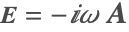 and E.
Discarding the displacement current ![]() from the Maxwell–Ampere law is the simplification that the magnetoquasistatics approximation employs. By not doing so, an electromagnetic wave equation will be modeled, as shown in the high-frequency section.
from the Maxwell–Ampere law is the simplification that the magnetoquasistatics approximation employs. By not doing so, an electromagnetic wave equation will be modeled, as shown in the high-frequency section.
High-frequency regime—Electromagnetic waves
If the characteristic size of the object ![]() approaches a fraction of the wavelength, say,
approaches a fraction of the wavelength, say, ![]() , or if none of the previous criteria was applicable, then the high-frequency regime needs to be considered and the full electromagnetic wave case needs to be solved.
, or if none of the previous criteria was applicable, then the high-frequency regime needs to be considered and the full electromagnetic wave case needs to be solved.
When working with high frequencies, energy is propagated through electromagnetic radiation. This type of radiation comprises synchronized oscillations of electric and magnetic fields, propagating through space to transport energy.
- Electromagnetic waves—Frequency domain: Describes harmonic electromagnetic waves in a high-frequency regime. In the frequency domain, a second-order wave equation is solved, given as:
where the dependent variable is the electric field intensity E. After solving the equation, one can compute the magnetic flux density ![]() in a subsequent step by using
in a subsequent step by using ![]() .
.
- Electromagnetic waves—Time domain: Describes time-varying electromagnetic waves. The time-dependent modeling of electromagnetic waves solves the following equation:
where the dependent variable is the magnetic vector potential ![]() .
.
Skin Depth
If fields vary in time, then the skin depth of the device with a given material is computed to decide which equations are appropriate to use. The value of the skin depth allows you to understand if it is possible to just consider the electric field or if the magnetic field also needs to be considered. The skin depth is directly related to a phenomenon known as skin effect and will be explained.
The skin depth ![]() [
[![]() ] compared to the characteristic size
] compared to the characteristic size ![]() [
[![]() ] will tell whether magnetic fields need to be considered or not:
] will tell whether magnetic fields need to be considered or not:
The skin depth is a measure of the depth to which an electromagnetic wave can penetrate a medium. The fact that the field intensity in a conductor decreases exponentially by its depth is knows as the skin effect. This effect describes the tendency of magnetic fields and associated alternating currents to be confined near the surface of a conductor and therefore limit the depth of penetration of the field. This means that when the skin depth ![]() is much larger than
is much larger than ![]() , if any magnetic field is present in a model, it does not affect the current flowing through the conductor.
, if any magnetic field is present in a model, it does not affect the current flowing through the conductor.
The skin depth ![]() is generally valid for any material medium, but conductors are where the concept of skin depth finds its most common application. For conductors, the skin depth
is generally valid for any material medium, but conductors are where the concept of skin depth finds its most common application. For conductors, the skin depth ![]() is approximated by the following equation:
is approximated by the following equation:
where ![]() is the angular frequency of the wave,
is the angular frequency of the wave, ![]() is the vacuum permeability,
is the vacuum permeability, ![]() is the relative permeability, and
is the relative permeability, and ![]() is the conductivity of the material. The skin effect is illustrated in the following figure.
is the conductivity of the material. The skin effect is illustrated in the following figure.

Figure 1. Distribution of current shown in a cross section of a circular conductor. For alternating currents, the current density decreases exponentially from the surface toward the center. The skin depth, ![]() , is defined as the depth at which the current density is just 1/e of the value at the conductor surface.
, is defined as the depth at which the current density is just 1/e of the value at the conductor surface.
The exponential drop of the magnitude of these fields can be expressed with the following proportionality:
where ![]() is the skin depth and
is the skin depth and ![]() is the penetration depth. So, in other words, the skin depth defines the distance across which the field strength is attenuated by a factor of
is the penetration depth. So, in other words, the skin depth defines the distance across which the field strength is attenuated by a factor of ![]() .
.
As an example, a closed loop of a copper wire will be used. The wire has a radius of ![]() [
[![]() ] and a loop radius of
] and a loop radius of ![]() [
[![]() ]. The closed loop is exposed to a uniform but variable frequency magnetic field. Copper has a relative permeability of
]. The closed loop is exposed to a uniform but variable frequency magnetic field. Copper has a relative permeability of ![]() and an electrical conductivity of
and an electrical conductivity of ![]() [
[![]() ]. The characteristic size
]. The characteristic size ![]() of the object would be the wire radius
of the object would be the wire radius ![]() [
[![]() ], and the skin depth
], and the skin depth ![]() will depend on
will depend on ![]() .
.
frequencies = {1, 10, 100, 1000, 10000};copperSkinDepth = PDEModels`SkinDepth[<|"RelativePermeability" -> 1, "ElectricalConductivity" -> 5.998 * 10 ^ 7|>, #]& /@ frequenciescopperSkinDepthRatio = 0.01 / copperSkinDepthPick[frequencies, Thread[copperSkinDepthRatio >= 1 / E]]Typically, for values of the skin depth-object size ratio ![]() greater than or equal to
greater than or equal to ![]() ,
, ![]() , it is recommended to consider both electric and magnetic fields.
, it is recommended to consider both electric and magnetic fields.
In this case of lower frequencies, like ![]()
![]() , the skin depth
, the skin depth ![]() is relatively large compared to the object size
is relatively large compared to the object size ![]() . In this case, an electroquasistatic analysis is sufficient.
. In this case, an electroquasistatic analysis is sufficient.
Frequency versus Time Domain
There are two types of analyses: the frequency domain and the time domain analysis. The time domain analysis is the most general analysis but also, computationally, the most expensive, so one prefers to avoid it. The time domain analysis is typically used when the excitation of the devices varies arbitrarily in time. The alternative is a frequency domain analysis.
To be able to make use of a frequency domain simulation, various aspects need to be satisfied. For one, the excitation of the device needs to be harmonic. Harmonic behavior is produced by a constant frequency alternating current (AC) input. Also, the response of the device needs to vary sinusoidally and remain at the same frequency. This last condition can only be met by systems with linear materials, where material properties remain constant with respect to field strength. All other cases will need a time-domain analysis.
In the time domain, fields can vary arbitrarily in time. A time-domain simulation is considered when dealing with nonlinear materials or when non-harmonic time-dependent inputs, such as isolated pulses, must be analyzed [Humphries, 2010].
Generally speaking, simulations in the time domain typically require more computational resources, such as time and computer memory, than frequency-domain or steady-state simulations.
Phasors
A field is referred to as time harmonic if it can be expressed as sine function with a specific frequency. An EM field is said to be time harmonic if the magnitude variation at any spatial position ![]() has a sinusoidal time dependence with an angular frequency
has a sinusoidal time dependence with an angular frequency ![]() .
.
A general expression of a harmonic electric field ![]() is written as:
is written as:
Here ![]() denotes the amplitude at the given position, and
denotes the amplitude at the given position, and ![]() is an initial phase shift at
is an initial phase shift at ![]() .
.
For analytical convenience, the time-harmonic relation (9) is often expressed in complex form known as the complex exponential representation (CER) or the phasor equation:
where ![]() is the imaginary unit, and the factor
is the imaginary unit, and the factor ![]() is equal to
is equal to ![]() .
.
By convention, the phasor is often expressed simply as:
in which it is implicitly interpreted that the real part of the complex-valued expression represents the real function ![]() .
.
The phasor can be understood as a rotating vector ![]() in the complex plane. The following figure illustrates this behavior.
in the complex plane. The following figure illustrates this behavior.

The rotating vector ![]() is known as the complex amplitude function. The amplitude function
is known as the complex amplitude function. The amplitude function ![]() rotates counterclockwise at a speed of the angular frequency
rotates counterclockwise at a speed of the angular frequency ![]() . At any given time
. At any given time ![]() , the projection of
, the projection of ![]() on the real axis represents the transient electric field
on the real axis represents the transient electric field ![]() , and the vector length
, and the vector length ![]() corresponds to the local amplitude.
corresponds to the local amplitude.
If the amplitude function and its complex conjugate are expressed as ![]() and
and ![]() , then the local amplitude
, then the local amplitude ![]() can be calculated by:
can be calculated by:
The use of phasors is only applicable for linear systems, so no material property can depend on the field under study. For materials that are nonlinear, the system must be solved in the time domain.
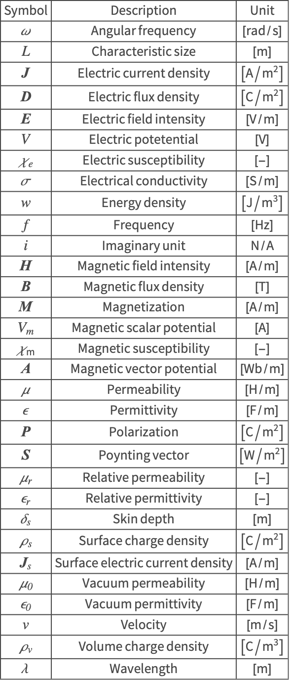
Nomenclature
References
1. Cardoso, J. R. (2018). Electromagnetics through the Finite Element Method. Boca Raton: CRC Press.
2. Humphries, S. (2010). Finite-Element Method for Electromagnetics. Field Precision LLC.
3. Jackson, J. D. (1999). Classical Electrodynamics. New York :Wiley.
4. Jin, J.-M. (2015). The Finite Element Method in Electromagnetics. John Wiley & Sons.
5. Sadiku, M. N. O. (2011). Elements of Electromagnetics (5th ed.). Oxford University Press.