Electrostatics
| Contents | Secondary Quantities |
| Introduction | Boundary Conditions in Electrostatics |
| Overview Example | Nomenclature |
| Electrostatic Equation | References |
Contents
Introduction
This monograph uses partial differential equations to model and analyze time-independent electric fields, electric potentials and charge densities distributions. The main assumption in an electrostatic simulation is that the electric and magnetic fields are not coupled.
The electrostatics equation is used to model electric fields produced by stationary charges. As a simplification of Maxwell's equations, it is only used to describe insulating or dielectric materials.
Modeling electromagnetic devices with partial differential equations (PDEs) is not the only way to model electromagnetic devices. Other techniques include setting up ordinary differential equations (ODEs). This approach is followed by the Wolfram System Modeler. Roughly speaking, the system modeler approach is more suitable for large systems of electromagnetic devices interacting, while the partial differential equation approach is more suitable for a fine-grained analysis of a specific device. In some cases, it is beneficial to use a combination of the two approaches.
The approach taken here is that in the introductory section a capacitor is used to introduce an electrostatic analysis and the functionality available. This will be followed by a more theoretical explanation of the underlying ideas and concepts. The theoretical background is much easier to understand once an intuition for the electrostatic analysis exists. After that, the available boundary conditions are discussed.
The equation used in this monograph is the electrostatic equation:
The goal of this electric device analysis is to find the potential distribution ![]() in units of volts
in units of volts ![]() under specific constraints. A subsequent step then finds secondary fields, such as the electric field intensity
under specific constraints. A subsequent step then finds secondary fields, such as the electric field intensity ![]() , and values such as the capacitance
, and values such as the capacitance ![]() . The analysis and interpretation of these physical quantities are useful to create a better quality engineering design of the device under consideration.
. The analysis and interpretation of these physical quantities are useful to create a better quality engineering design of the device under consideration.
The modeling process as such results in a system of partial differential equations (PDEs) that can be solved with NDSolve.
Extended examples of electromagnetic modeling can be found in the Model Collection.
The electromagnetic device analysis is typically done in stages. First, for the object to be analyzed, a geometric model needs to be created. The geometric model is typically created within a computer-aided design (CAD) process. CAD models can either be imported or created in product. To import geometries, common file formats like DXF, STL or STEP are supported. These geometries can be imported with Import. The alternative is to create the geometrical models in product, for example, by using OpenCascadeLink.
Once the geometric model is made available, some thought needs to be put into what type of analysis is to be performed. The next step is the setup of boundary conditions and constraints. Materials to be used further specify the PDE model. Once the PDE model is fully specified, the subsequent finite element analysis will then compute the desired quantities of the device under investigation. These quantities are then post-processed, either by visualizing them or some derived quantities are computed. This tutorial shows the necessary steps for everything except the CAD model generation.
Electromagnetic devices are typically three-dimensional objects. For the models, special cases exist that result in simplified 2D models. In fact, 2D models have been known to solve 90% of the important problems in electrical engineering [Cardoso, 2018].
The symbols and corresponding units used throughout this tutorial are summarized in the Nomenclature section.
Overview Example
To illustrate the usage of the finite element method in these subcases of electromagnetics, it is instructive to present a simple example and give an overview of the setup, various analysis types and post-processing steps possible.
Needs["NDSolve`FEM`"]
$HistoryLength = 0;
The first example is to introduce the workflow of setting up a simple electromagnetics PDE model, which will cover an electrostatic analysis.
Consider the following setup: a 3D circular parallel capacitor composed of two conductive plates with a dielectric material in between.

Depiction of a 3D capacitor and the cross section of the dielectric region in blue, its height ![]() and radius
and radius ![]() .
.
To keep the model simple, only the dielectric region, shown in blue, will be modeled.
Creating an electromagnetics model always comprises the same steps:
Geometry
When a capacitor device is modeled, there are two possible ways to model it. One is to consider the device and the surrounding volume. In this approach, one can simulate the field that appears at the edge of the plates and extends away outside from the device into the surrounding volume considered. This field is known as the fringing field. The second approach, used here, considers the dielectric region. For more details on which approach to use and what the effects on the model are, refer to the capacitance section.
r0 = 0.01;
h = 0.001;Ω = Cylinder[{{0, 0, 0}, {0, 0, h}}, r0];Region[Ω]One thing to keep in mind is the scale used in the geometric model. If the length of the boundary mesh is, for example, in units of meters then the material parameters will need to be specified in consistent units.
More information on generating or importing 3D geometric models can be found in the Using OpenCascadeLink tutorial.
Material Parameters
The next step is to assign material parameters. Generally, all parameters for an electromagnetics model are collected in an Association pars that includes the necessary parameter values.
The default vacuum permittivity value ![]() is used throughout the whole monograph. The "VacuumPermittivity" parameter can also be specified if the constant should have a different value, like 1, to scale the equation.
is used throughout the whole monograph. The "VacuumPermittivity" parameter can also be specified if the constant should have a different value, like 1, to scale the equation.
In this model, the dielectric of the capacitor will have a relative permittivity of ![]() . This value is just representing a general dielectric material.
. This value is just representing a general dielectric material.
pars = <|"RelativePermittivity" -> 2|>;Specifying a material as an Entity directly is currently not possible.
Material parameters where the values are given as Quantity objects can be used. The exact property names to specify material properties needed can be found on the reference pages of ElectrostaticPDEComponent.
Geometries consisting of several materials can also be used, and an example of such a use case is presented in the section on multiple materials of electrostatics.
Units
Should the units of the geometry be different from the material units, then the material units can be scaled.
<|"RelativePermittivity" -> 2, "VacuumPermittivity" -> Quantity[8.854187813*^-12, "Farads"/"Meters"], "ScaleUnits" -> {"Meters" -> "Millimeters"}|>;Internally, all material data units are converted to "SIBase" units. As a consequence, the default unit of length is "Meters". If the units of the geometry are also in meters, then nothing needs to be changed. If the units of the geometry are not in meters, then either the PDE and material properties need to be scaled to the units of the geometry or the geometry needs to be scaled to "Meters". To scale the units of the PDE and material parameters, the parameter "ScaleUnits" can be given. If not explicitly stated otherwise, examples in this tutorial use the default "SIBase" units.
Boundary Conditions
Boundary conditions must be defined at physical boundaries to fully specify the problem. In this case, the device will be charged by applying a voltage difference between the plates. In essence, this is done by applying a DirichletCondition or NeumannValue at the terminals, respectively. Various boundary conditions can be used and will be discussed in more detail in the Boundary conditions in electrostatics section. For the purpose of this overview, an electric potential condition will be sufficient.
The purpose of this section is to establish the positions where the boundary conditions are to be applied.
A way to find the positions where the boundary conditions are applied is to visualize them together with the outline geometry defined previously in the geometry section.
upperPlate = z == h;Show[Graphics3D[{Opacity[0.2], Ω}, Boxed -> False], ...]The same applies for the lower plate.
lowerPlate = z == 0;contour = (x ^ 2 + y ^ 2 == r0 ^ 2) && (0 < z < h);
Show[Graphics3D[{Opacity[0.2], Ω}, Boxed -> False], ...]On the side of the dielectric, a zero NeumannValue is present. A zero NeumannValue boundary condition is the default if nothing else is specified, allowing that boundary condition to be omitted.
For more complicated geometries, a different technique to specify boundary condition predicates may be appropriate and it can be seen in the Spherical Capacitor tutorial.
Mesh Generation
To perform a finite element analysis, the geometric region needs to be discretized into a mesh.
mesh = ToElementMesh[Ω];More information about the mesh generation process can be found in the ElementMesh generation tutorial. Another option is to import a mesh. Some common mesh file formats can be imported with the help of the FEMAddOns.
Electrostatic Analysis
An electrostatic analysis will seek the electric potential and electric field distribution inside the dielectric due to the static charge distribution imposed on the model. The dependent variable is the electric potential ![]() .
.
An electrostatic analysis in effect solves:
where ![]() is the vacuum permittivity and
is the vacuum permittivity and ![]() is the relative permittivity. This equation is provided by the function ElectrostaticPDEComponent.
is the relative permittivity. This equation is provided by the function ElectrostaticPDEComponent.
vars = {V[x, y, z], {x, y, z}};op = ElectrostaticPDEComponent[vars, pars]By specifying the relative permittivity ![]() , the function generates the equation based on this linear constitutive relation. Others parameters, such as a polarization vector
, the function generates the equation based on this linear constitutive relation. Others parameters, such as a polarization vector ![]() , can be specified.
, can be specified.
Subscript[Γ, ground] = ElectricPotentialCondition[lowerPlate, vars, pars, <|"ElectricPotential" -> 0|>]V0 = 1;
Subscript[Γ, potential] = ElectricPotentialCondition[upperPlate, vars, pars, <|"ElectricPotential" -> V0|>]Vfun = NDSolveValue[{op == 0, Subscript[Γ, ground], Subscript[Γ, potential]}, V, {x, y, z}∈mesh]The result is an InterpolatingFunction object, which gives the electric potential distribution ![]() .
.
More information about the solution process and its options can be found in the NDSolve Options for Finite Elements tutorial.
Post-processing
The primary solution of the electrostatics PDE model is the electric potential.
SliceDensityPlot3D[Vfun[x, y, z], "CenterPlanes", {x, y, z}∈mesh, BoxRatios -> {4, 1, 1}, ...]Also of interest are the electric field intensity ![]() and the electric flux density
and the electric flux density ![]() , from which the capacitance value
, from which the capacitance value ![]() can be obtained. These fields are recovered from the electric potential. More details about how to compute capacitance values are shown in the Capacitance section.
can be obtained. These fields are recovered from the electric potential. More details about how to compute capacitance values are shown in the Capacitance section.
Efield = -Grad[Vfun[x, y, z], {x, y, z}]For a three-dimensional model, the function Grad returns a list of three InterpolatingFunction instances with the three independent variables ![]() ,
, ![]() and
and ![]() each.
each.
Efield /. {x -> 0, y -> 0, z -> 0}Various components of the electric field can be accessed by using Part.
Efield[[3]]With the electric field intensity ![]() computed, the capacitance of the capacitor can be found with:
computed, the capacitance of the capacitor can be found with:
where ![]() in units of
in units of ![]() is the charge's magnitude held on one of the plates of the capacitor,
is the charge's magnitude held on one of the plates of the capacitor, ![]() is the potential difference between the plates, and
is the potential difference between the plates, and ![]() is the normal component of the electric flux density at one of the plates.
is the normal component of the electric flux density at one of the plates.
One must first compute the voltage at the upper plate to compute the potential difference between the plates. The upper voltage is obtained by integrating ![]() over the disk area and dividing it by the same area.
over the disk area and dividing it by the same area.
Vupper = (NIntegrate[V0, {x, y}∈Disk[{0, 0}, r0]]/NIntegrate[1, {x, y}∈Disk[{0, 0}, r0]])By definition, at ground, a potential of 0 is always used.
ΔV = Vupper - 0;In this case, the inward normal component at the upper plate is the ![]() component in the negative direction
component in the negative direction ![]() . The
. The ![]() component is given by
component is given by ![]() .
.
To calculate ![]() , extracting the vacuum permittivity value used in the model is necessary. Ensuring consistency in values throughout a computation involves using the default model parameter computation.
, extracting the vacuum permittivity value used in the model is necessary. Ensuring consistency in values throughout a computation involves using the default model parameter computation.
pars = PDEModels`DefaultModelParameters[vars, pars, "Electrostatics"];ϵ0 = pars["VacuumPermittivity"];
ϵr = pars["RelativePermittivity"];Dz = ϵ0 * ϵr * Efield[[3]] /. {z -> h};Q0 = NIntegrate[-Dz, {x, y}∈Disk[{0, 0}, r0]]C0 = Abs[Q0] / ΔVFor this example, an analytical solution of the value of the expected capacitance is available.
CAnalytical = (ϵ0 * 2π * r0^2/h)The numerical capacitance obtained is in good agreement with the analytical one.
100 * (Abs[C0 - CAnalytical]/CAnalytical)In the above case, the symbolic region representation Disk was used as the upper part of the cylindrical region ![]() . In real-world applications, a symbolic representation of the boundary in question may not always be readily available. Even if a boundary representation is available, it may differ from the numeric representation used during the computation. This discrepancy arises because a mesh is only an approximation to the symbolic representation, such as the Disk. For this reason, it may generally be beneficial to directly use the numerical approximation of the region in question. This can be done by using FEMNBoundaryIntegrate.
. In real-world applications, a symbolic representation of the boundary in question may not always be readily available. Even if a boundary representation is available, it may differ from the numeric representation used during the computation. This discrepancy arises because a mesh is only an approximation to the symbolic representation, such as the Disk. For this reason, it may generally be beneficial to directly use the numerical approximation of the region in question. This can be done by using FEMNBoundaryIntegrate.
When using FEMNBoundaryIntegrate, one needs to specify the element marker of the desired boundary surface. In this case , the number 2 refers to the upper plate boundary. For more information on markers in a mesh, see the section Markers in the element mesh generation tutorial.
Subscript[ΔV, FEM] = ((FEMNBoundaryIntegrate[V0, {x, y, z}, mesh, ElementMarker == 2]/FEMNBoundaryIntegrate[1, {x, y, z}, mesh, ElementMarker == 2]) - 0);C0 = Abs[FEMNBoundaryIntegrate[-ϵ0 * ϵr * Efield[[3]], {x, y, z}, mesh, ElementMarker == 2]] / Subscript[ΔV, FEM]100 * (Abs[C0 - CAnalytical]/CAnalytical)While the error with the numerical mesh is larger than with the symbolic surface region, it is still acceptable. The use of FEMNBoundaryIntegrate is convenient because it is a generally usable workflow when no symbolic representation of the surface in question is available.
As yet another alternative method, one can compute the capacitance by means of the electrostatic energy ![]() :
:
where ![]() is given by a volume integral:
is given by a volume integral:
Dfield = ϵ0 * ϵr * Efield;We = NIntegrate[(1/2) * Dfield.Efield, {x, y, z}∈mesh]Here, the mesh of the region ![]() has been used.
has been used.
C0 = (2We/ΔV^2)100 * (Abs[C0 - CAnalytical]/CAnalytical)Details about the methods employed to compute the capacitance are shown in the Capacitance section.
Electrostatic Equation
This section gives an introduction to modeling electrostatics models.
Electrostatics is the subfield of electromagnetics that deals with electric fields produced by static charges. So, the driving force behind the generated electric field is distributed charges or a specified potential difference ![]() in units of volts
in units of volts ![]() . The electrostatic equation, which is derived from Maxwell's equations, is used for modeling steady electric fields produced by static charges within an insulating or dielectric material. Here, the most general form of the equation within a dielectric medium is shown:
. The electrostatic equation, which is derived from Maxwell's equations, is used for modeling steady electric fields produced by static charges within an insulating or dielectric material. Here, the most general form of the equation within a dielectric medium is shown:
The dependent variable in this equation is the electric potential ![]() , which varies with position
, which varies with position ![]() . The equation is made up of a diffusive term
. The equation is made up of a diffusive term ![]() with the vacuum permittivity
with the vacuum permittivity ![]() as the diffusion coefficient, and a derivative term
as the diffusion coefficient, and a derivative term ![]() in which the variable
in which the variable ![]() is the polarization vector. The term
is the polarization vector. The term ![]() in units of
in units of ![]() denotes a volume charge density within the domain, and it is explained in the Source Types section.
denotes a volume charge density within the domain, and it is explained in the Source Types section.
Note that metallic components in the domain cannot be considered with this equation; this equation is for dielectric or insulating material only, because for conducting material there is no potential difference. This means that electrodes, for example, have to be modeled as boundary conditions. Also, any metal inside the domain needs to be removed.
The electrostatic equation can be solved for 1D axisymmetric, 1D, 2D, 2D axisymmetric and 3D models.
Model setup
The inputs needed for an electrostatic model are:
Next, examples for setting up the equations are provided.
ElectrostaticPDEComponent[{V[x, y, z], {x, y, z}}, <|"VacuumPermittivity" -> Subscript[ϵ, 0] * IdentityMatrix[3]|>]For 2D models, there exists a special case of symmetry where the electric potential varies only in the ![]() and
and ![]() directions and is constant in the
directions and is constant in the ![]() direction. With this symmetry, a similar equation is solved, with the exception that a thickness variable
direction. With this symmetry, a similar equation is solved, with the exception that a thickness variable ![]() denoting thickness in the
denoting thickness in the ![]() direction is added:
direction is added:
ElectrostaticPDEComponent[{V[x, y], {x, y}}, <|"VacuumPermittivity" -> Subscript[ϵ, 0] * IdentityMatrix[2], "Thickness" -> d|>]The default value for the thickness is ![]() .
.
Just as there can be a symmetry when simulating in the ![]() -
-![]() plane, a symmetry can exist in 1D models. In a 1D electrostatic model, a cross-sectional area
plane, a symmetry can exist in 1D models. In a 1D electrostatic model, a cross-sectional area ![]() , which represents the
, which represents the ![]() and
and ![]() directions, is added to the equation:
directions, is added to the equation:
The default value for the cross-sectional area is ![]() .
.
ElectrostaticPDEComponent[{V[x], {x}}, <|"VacuumPermittivity" -> Subscript[ϵ, 0] * IdentityMatrix[1], "CrossSectionalArea" -> A|>]The 1D and 2D axisymmetric models take into account another type of symmetry that is observed in 3D solids, which have an axis of revolution. For more details on these cases, see the section Axisymmetric models.
Note that this model definition uses inactive PDE operators. "Numerical Solution of Partial Differential Equations" has several sections that explain the use of inactive operators.
Electrostatics
As the name electrostatic suggests, this subcase deals with electric fields that do not vary in time, and thus the fields are called static. To simplify, vacuum will be assumed as the simulation domain.
An electrostatics case will be described by two of Maxwells's equations—Gauss's law:
and Faraday's law without the magnetic induction term:
Gauss's law (Eqn. 1) states that the divergence of the electric field intensity ![]() at any point in space is proportional to the volume charge density
at any point in space is proportional to the volume charge density ![]() at that point. In other words, the charge density influences the behavior of
at that point. In other words, the charge density influences the behavior of ![]() in that region. The divergence for the electric field
in that region. The divergence for the electric field ![]() will tell you how much the electric field is spreading out or converging at any point in space.
will tell you how much the electric field is spreading out or converging at any point in space.
On the other hand, Faraday's law (Eqn. 2) states that ![]() is curl-free and therefore a conservative vector field. This equation enables the derivation of the scalar electric potential
is curl-free and therefore a conservative vector field. This equation enables the derivation of the scalar electric potential ![]() .
.
Using the properties of field operators, the following equation can be deduced:
This equation states that the curl of the gradient of any scalar function ![]() is zero. Thus, by comparing both equations and substituting the electric field
is zero. Thus, by comparing both equations and substituting the electric field ![]() in Eqn. 3, it can be deduced that
in Eqn. 3, it can be deduced that ![]() can be represented as the gradient of a function
can be represented as the gradient of a function ![]() .
.
The negative sign was placed by convenience and for historical reasons.
Now, by substituting Eqn. 4 in Eqn. 5, one can obtain the electrostatic equation in free space:
Dielectric materials and the constitutive equation
The above equation is valid in vacuum. The electrostatic equation in vacuum can be extended to consider dielectric materials. Dielectric materials are distinguished from conductors by not having any free electrons; instead, charges in dielectric material are bounded by forces. When an external electric field is applied to a dielectric material, dipole moments are induced because the electron clouds in the atoms are displaced in the opposite direction of the ![]() field and the nuclei are displaced from their equilibrium positions in the same direction as the
field and the nuclei are displaced from their equilibrium positions in the same direction as the ![]() field points to.
field points to.
This displacement of charges creates a bound volume charge density ![]() , and in consequence a vector field
, and in consequence a vector field ![]() , which expresses the density of permanent or induced electric dipole moments. Due to this polarization vector, the electric field inside a dielectric material will be different from the one in free space [Sadiku, 2011].
, which expresses the density of permanent or induced electric dipole moments. Due to this polarization vector, the electric field inside a dielectric material will be different from the one in free space [Sadiku, 2011].

On the left: a nonpolar atom. To the right: polarization of a nonpolar atom when an electric field ![]() is applied.
is applied.
The polarization vector ![]() and the bound volume charge density
and the bound volume charge density ![]() are related by the following equation:
are related by the following equation:
which resembles Gauss's law. The negative sign arises due to the opposite signs on the charges in the aligned dipoles of the dielectric, which are induced by the external ![]() field.
field.
It is important to understand how the bound charges of a dielectric interact with the external electric field applied to it. Distinguishing between the free charges and the bound charges that constitute the dielectric itself is helpful. Free charges, denoted as ![]() , can be introduced to or removed from a conductor, such as a capacitor plate. In contrast, bound charges are immobile within the dielectric.
, can be introduced to or removed from a conductor, such as a capacitor plate. In contrast, bound charges are immobile within the dielectric.
In a system where both free and bound charge densities are present, Gauss's law needs to be modified to include the total charge density:
By substituting Eqn. 6 into Eqn. 7, the result is:
which can be further simplified by introducing a new quantity ![]() , whose name is the electric flux density:
, whose name is the electric flux density:
The electric flux density ![]() is defined as:
is defined as:
This constitutive relation basically says that the application of an external electric field ![]() to a dielectric material causes the flux density to be greater than it would be in free space. In free space,
to a dielectric material causes the flux density to be greater than it would be in free space. In free space, ![]() .
.
Substituting Eqn. 8 into Eqn. 9 yields the electrostatic equation:
ElectrostaticPDEComponent[{V[x, y], {x, y}}, <|"VacuumPermittivity" -> Subscript[ϵ, 0] * IdentityMatrix[2], "Polarization" -> {Px[x, y], Py[x, y]}|>]Linear dielectric materials
For linear materials, ![]() can be described in terms of the electric field as
can be described in terms of the electric field as ![]() , where the unitless
, where the unitless ![]() is the electric susceptibility of the material. So, for linear materials, the constitutive relations are:
is the electric susceptibility of the material. So, for linear materials, the constitutive relations are:
where the unitless ![]() is the relative permittivity given by:
is the relative permittivity given by:
and ![]() is the absolute permittivity. Note that for free space
is the absolute permittivity. Note that for free space ![]() . On the other hand, a material is said to be nonlinear if
. On the other hand, a material is said to be nonlinear if ![]() does not vary linearly with
does not vary linearly with ![]() .
.
ElectrostaticPDEComponent[{V[x, y], {x, y}}, <|"VacuumPermittivity" -> Subscript[ϵ, 0], "RelativePermittivity" -> Subscript[ϵ, 𝓇] * IdentityMatrix[2]|>]The relative permittivity can depend on the space coordinate ![]() and vary in the region considered, i.e. an inhomogeneous material, or vary with direction, i.e. an anisotropic material.
and vary in the region considered, i.e. an inhomogeneous material, or vary with direction, i.e. an anisotropic material.
Multiple materials
It is common to model different materials in the simulation domain, for example, if one wants to simulate the electric field that extends beyond a capacitor into the surrounding space. This field is known as the fringing field. To simulate the fringing field of a capacitor, one needs to include the dielectric region and the air surrounding it.
Here, a cross section of a parallel capacitor is modeled, assuming that the electrodes extend along both directions of the ![]() axis, perpendicular to the
axis, perpendicular to the ![]() -
-![]() plane. This model will aid in illustrating energy, capacitance and force calculations in future sections.
plane. This model will aid in illustrating energy, capacitance and force calculations in future sections.

Cross section of a parallel capacitor surrounded by vacuum.
Additionally, in this example, element markers will be used to denote the relative permittivity values for each subregion and to specify the boundary conditions. The concept of element markers and their application in meshes is detailed in the Element Marker section of the Element Mesh generation tutorial.
LC = 2;
wdC = 0.5;
d0C = 0.1;
thC = 0.4 * d0C;bmeshC = ToBoundaryMesh["Coordinates" -> {{-LC / 2, -LC / 2}, {LC / 2, -LC / 2}, {LC / 2, LC / 2}, {-LC / 2, LC / 2}, {-wdC / 2, -d0C - thC}, {wdC / 2, -d0C - thC}, {wdC / 2, -d0C}, {-wdC / 2, -d0C}, {-wdC / 2, d0C}, {wdC / 2, d0C}, {wdC / 2, d0C + thC}, {-wdC / 2, d0C + thC}}, "BoundaryElements" -> {LineElement[{{1, 2}, {2, 3}, {3, 4}, {4, 1}, {5, 6}, {6, 7}, {7, 8}, {8, 5}, {9, 10}, {10, 11}, {11, 12}, {12, 9}, {7, 10}, {8, 9}}, {1, 1, 1, 1, 2, 2, 2, 2, 3, 3, 3, 3, 4, 4}]}];regionMarkersC = <|"dielectric" -> 1, "air" -> 2|>;Next, region markers with the "RegionMarker" option of ToElementMesh are specified. To do so, a coordinate within the dielectric and the air region should be given, as well as an integer marker. Optionally, an additional maximum cell measure can be specified to refine a subregion. The most accurate and efficient method to deal with multiple material regions is by element makers, as then the mesh will have a specific subregion for the material, which will result in an accurate solution.
Remember that metals should be removed from the mesh when they are inside the domain of analysis.
meshC = ToElementMesh[bmeshC, "RegionHoles" -> {{0, d0C + thC}, {0, -d0C - thC}}, "RegionMarker" -> {{{0, 0}, regionMarkersC["dielectric"]}, {{0, LC / 4}, regionMarkersC["air"]}}, MaxCellMeasure -> 0.003];varsC = {V[x, y], {x, y}};The air region has a relative permittivity of ![]() , while the dielectric region has a value of
, while the dielectric region has a value of ![]() .
.
parsC = <|"RelativePermittivity" -> Piecewise[{{7, ElementMarker == regionMarkersC["dielectric"]}}, 1]|>;See this note about the setup of efficient PDE coefficients.
opC = ElectrostaticPDEComponent[varsC, parsC]In this capacitor, the upper electrode will have an electric potential of ![]() and the lower electrode will be grounded. In addition to these boundary conditions, a zero surface charge density is applied to the box boundaries; this will constrain the electric field to remain inside the box.
and the lower electrode will be grounded. In addition to these boundary conditions, a zero surface charge density is applied to the box boundaries; this will constrain the electric field to remain inside the box.
A zero surface charge density is equivalent to a Neumann zero value, and as these are the natural default boundary conditions, they can be left out.
In this model, markers are used in the boundary condition specification. As these are DirichletCondition boundaries, point element markers are used.
meshC["PointElementMarkerUnion"]The element markers for the lower and upper electrodes are ![]() and
and ![]() , respectively.
, respectively.
Subscript[Γ, groundC] = ElectricPotentialCondition[ElementMarker == 2, varsC, parsC, <|"ElectricPotential" -> 0|>];V0C = 1*^4;
Subscript[Γ, potentialC] = ElectricPotentialCondition[ElementMarker == 3, varsC, parsC, <|"ElectricPotential" -> V0C|>];pdeC = {opC == 0, {Subscript[Γ, groundC], Subscript[Γ, potentialC]}};VfunC = NDSolveValue[pdeC, V, {x, y}∈meshC];Next, the computation of the electric field intensity ![]() and the electric flux density
and the electric flux density ![]() will be carried out to observe their behavior.
will be carried out to observe their behavior.
To correctly compute the electric field ![]() and
and ![]() , one has to take into account that at interfaces between different materials there can be discontinuities. To see details about the conditions at interfaces, refer to the section Boundary Conditions in Electrostatics.
, one has to take into account that at interfaces between different materials there can be discontinuities. To see details about the conditions at interfaces, refer to the section Boundary Conditions in Electrostatics.
To address this discontinuity, DiscontinuousInterpolatingFunction or EvaluateOnElementMesh can be used. These functions will prioritize the value from one of the subregions. The default uses the order given in "MeshElementMarkerUnion". To specify a priority, you can give an option "MarkerPriority".
meshC["MeshElementMarkerUnion"]At the dielectric/air interface, the default in this case will prioritize the dielectric region of the capacitor over the air. In this example, a discontinuity in ![]() can be seen at the interface.
can be seen at the interface.
Since the electric field intensity ![]() is the gradient of the electric potential
is the gradient of the electric potential ![]() , a DiscontinuousInterpolatingFunction will be used first in the electric potential function and then the derivative will be computed from the new discontinuous function.
, a DiscontinuousInterpolatingFunction will be used first in the electric potential function and then the derivative will be computed from the new discontinuous function.
The DiscontinuousInterpolatingFunction is very useful when one tries to compute values at the interface between two different materials and then use them for plots or as arguments for other computations.
VfunCDIF = DiscontinuousInterpolatingFunction[VfunC]The output is a DiscontinuousInterpolatingFunction, where it first shows the domain bounds and then the marker priority.
EfieldC = -Grad[VfunCDIF[x, y], {x, y}]Show[VectorPlot[EfieldC, {x, y}∈meshC, ...], bmeshC["Wireframe"]]The vector plot visualizes that the zero Neumann values at the boundaries restrain the field lines to remain within the domain. In other words, the field is forced to be tangential to the exterior boundaries. This constraint in the field has a direct influence in the central part of the field and consequently in the capacitance value that is computed and discussed in the Capacitance section.
Since the model has two different values for the relative permittivity ![]() , EvaluateOnElementMesh must be used to correctly calculate the electric flux density
, EvaluateOnElementMesh must be used to correctly calculate the electric flux density ![]() in the different material regions. The electric flux also will be represented with a DiscontinuousInterpolatingFunction.
in the different material regions. The electric flux also will be represented with a DiscontinuousInterpolatingFunction.
parsC = PDEModels`DefaultModelParameters[varsC, parsC, "Electrostatics"];
ϵ0 = parsC["VacuumPermittivity"];
ϵr = parsC["RelativePermittivity"];DfieldC = Through[EvaluateOnElementMesh[{x, y}, ϵ0 * ϵr * EfieldC, meshC][x, y]]EvaluateOnElementMesh returns a list of discontinuous interpolating functions. These interpolating functions do not have the independent variables ![]() and
and ![]() attached. Adding them is trivial with the Through command.
attached. Adding them is trivial with the Through command.
To observe the discontinuity in electric flux density, one can create a DensityPlot of the magnitude of the electric flux density. Sometimes, it is necessary to extract the maximum and minimum values of the plotted variable. Therefore, a rule will be created that allows extraction of the "ValuesOnGrid" of the fields, followed by applying MinMax.
getValuesOnGrid = (head : DiscontinuousInterpolatingFunction | InterpolatingFunction)[a__][d__] :> head[a]["ValuesOnGrid"];DfieldNormRange = MinMax[Sqrt[DfieldC[[1]]^2 + DfieldC[[2]]^2] /. getValuesOnGrid ]DensityPlot[Sqrt[DfieldC[[1]] ^ 2 + DfieldC[[2]] ^ 2], {x, y}∈ meshC, ...]Anisotropic dielectric materials
Dielectrics can be either isotropic or anisotropic. Isotropic materials are materials that have the same electric properties in all directions. For an isotropic ![]() ,
, ![]() and
and ![]() always have the same direction due to the relation
always have the same direction due to the relation ![]() . In anisotropic materials, the relative permittivity becomes a tensor
. In anisotropic materials, the relative permittivity becomes a tensor ![]() and the electric properties change with direction. Crystalline materials are, for example, anisotropic [Sadiku, 2011].
and the electric properties change with direction. Crystalline materials are, for example, anisotropic [Sadiku, 2011].
For anisotropic materials, ![]() or
or ![]() are now tensors. In the 3D case, the relative permittivity is then a three-by-three tensor that has nine components:
are now tensors. In the 3D case, the relative permittivity is then a three-by-three tensor that has nine components:
where ![]() is the relative permittivity tensor.
is the relative permittivity tensor. ![]() and
and ![]() are called the principal permittivity coefficients and off-diagonal permittivity coefficients, respectively.
are called the principal permittivity coefficients and off-diagonal permittivity coefficients, respectively.
With a relative permittivity as tensor, the relation between ![]() and
and ![]() changes to
changes to ![]() . This has the consequence that
. This has the consequence that ![]() and
and ![]() are no longer parallel.
are no longer parallel.
ElectrostaticPDEComponent[{V[x, y], {x, y}}, <|"VacuumPermittivity" -> Subscript[ϵ, 0], "RelativePermittivity" -> {{Subscript[ϵ, xx], Subscript[ϵ, xy]}, {Subscript[ϵ, yx], Subscript[ϵ, yy]}}|>]In the following example, an electro-optic modulator (EOM) is modeled. This EOM consists of a lithium niobate core (![]() ), a silica cladding (
), a silica cladding (![]() ) and two gold electrodes, which work as capacitor, that induce an electric field in the core. EOMs are used widely in many different photonic devices.
) and two gold electrodes, which work as capacitor, that induce an electric field in the core. EOMs are used widely in many different photonic devices.
The lithium niobate core is an optical waveguide where the light passes through. This material is an orthotropic material. The material is symmetric along the principal directions ![]() and
and ![]() , and the off-diagonal permittivity coefficients are zero. The permittivity tensor for this case is:
, and the off-diagonal permittivity coefficients are zero. The permittivity tensor for this case is:
The design of this EOM consists of a trapezoidal ![]() waveguide, resting on an
waveguide, resting on an ![]() plate, and two golden electrodes, placed above the core, that are embedded in a silica cladding. This design is based on [Loucas, 2023].
plate, and two golden electrodes, placed above the core, that are embedded in a silica cladding. This design is based on [Loucas, 2023].

Cross section of an electro-optical modulator. The electrodes are in yellow, the silica cladding in gray and the LiNbO3 plate and waveguide in purple.
In this model, the electric field ![]() induced by the electrodes is simulated. Due to axial symmetry around the
induced by the electrodes is simulated. Due to axial symmetry around the ![]() axis and with the assumption that the EOM is sufficiently long, the electric field, has no dependence on
axis and with the assumption that the EOM is sufficiently long, the electric field, has no dependence on ![]() . This allows you to simplify the model and just model the cross-sectional area of the EOM.
. This allows you to simplify the model and just model the cross-sectional area of the EOM.
thE = 1*^-6;
wdE = 8.5*^-6;
topGap = 5*^-6;
baseGap = 8*^-6;thbSiO2 = 3.2*^-6;
wdSiO2 = 20*^-6 + baseGap;
thSiO2 = 1.5*^-6;
hSiO2 = 5*^-6;wdLiN = 0.6wdSiO2;
thLiN = 0.25*^-6;
ht = 0.35*^-6;
ca = ht / Tan[70Degree];
lt = 1.2*^-6;
l1 = lt / 2 - ca;
l2 = -lt / 2 + ca;bmeshEOM = ToBoundaryMesh[...];As two different materials are being modeled, a region marker should be used to define the subregions.
regionMarkersEOM = <|"LiNbO3" -> 1, "SiO2" -> 2|>;meshEOM = ToElementMesh[bmeshEOM, "RegionHoles" -> {{-wdE, thE / 2}, {wdE, thE / 2}}, "RegionMarker" -> {{{0, 0}, regionMarkersEOM["LiNbO3"]}, {{0, -thbSiO2 / 2}, regionMarkersEOM["SiO2"]}}];varsEOM = {V[x, y], {x, y}};
parsEOM = <|"VacuumPermittivity" -> 8.85418781*^-18, "RelativePermittivity" -> {{Piecewise[{{43.6, ElementMarker == regionMarkersEOM["LiNbO3"]}}, 3.9], 0}, {0, Piecewise[{{29.16, ElementMarker == regionMarkersEOM["LiNbO3"]}}, 3.9]}}|>;ϵLiNbO3 = {{43.6, 0}, {0, 29.16}};
ϵSiO2 = {{3.9, 0}, {0, 3.9}};opEOM = ElectrostaticPDEComponent[varsEOM, parsEOM]The potential difference between the electrodes is of ![]() , with
, with ![]() on the boundaries of the right-positive electrode and
on the boundaries of the right-positive electrode and ![]() on the left-negative electrode.
on the left-negative electrode.
In this model, markers are used in the boundary condition specification. As these are DirichletCondition boundaries, point element markers are used.
meshEOM["PointElementMarkerUnion"]The element markers for the left and right electrodes are 3 and 4, respectively.
V0EOM = 1;
Subscript[Γ, p1] = ElectricPotentialCondition[ElementMarker == 3, varsEOM, parsEOM, <|"ElectricPotential" -> -V0EOM / 2|>];Subscript[Γ, p2] = ElectricPotentialCondition[ElementMarker == 4, varsEOM, parsEOM, <|"ElectricPotential" -> V0EOM / 2|>];pdeEOM = {opEOM == 0, {Subscript[Γ, p1], Subscript[Γ, p2]}};VfunEOM = NDSolveValue[pdeEOM, V, {x, y}∈meshEOM];VfunEOMDIF = DiscontinuousInterpolatingFunction[VfunEOM]EfieldEOM = -Grad[VfunEOMDIF[x, y], {x, y}];Show[VectorPlot[EfieldEOM, {x, y}∈meshEOM, AspectRatio -> Automatic, RegionFillingStyle -> None, RegionBoundaryStyle -> None, Frame -> False, VectorPoints -> Fine], bmeshEOM["Wireframe"]]Nonlinear dielectric materials
For nonlinear materials, the relationship between the electric field intensity ![]() and the electric flux density
and the electric flux density ![]() changes to:
changes to:
where ![]() is the polarization when no electric field is present, known as the remanent polarization vector.
is the polarization when no electric field is present, known as the remanent polarization vector.
This equation takes into account the linear relationship ![]() as well as the additional polarization caused by Pr. In simple terms, the remanent polarization contributes to the overall electric flux density even in the absence of an external electric field.
as well as the additional polarization caused by Pr. In simple terms, the remanent polarization contributes to the overall electric flux density even in the absence of an external electric field.
The use of the constitutive relation expressed in Eqn. 10 is limited to nonlinear materials that do not show hysteresis effects, such as ferroelectrics.
ElectrostaticPDEComponent[{V[x, y], {x, y}}, <|"VacuumPermittivity" -> Subscript[ϵ, 0], "RelativePermittivity" -> Subscript[ϵ, 𝓇], "RemanentPolarization" -> {Prx[x, y], Pry[x, y]}|>]Axisymmetric models
An axisymmetric simulation can be performed when a 3D solid has an axis of revolution. An axisymmetric model uses a truncated cylindrical coordinate system in 2D with independent variables ![]() instead of the cylindrical coordinates
instead of the cylindrical coordinates ![]() . The cylindrical coordinate variable
. The cylindrical coordinate variable ![]() disappears because the system is rotationally symmetric about the
disappears because the system is rotationally symmetric about the ![]() axis.
axis.
The 2D axisymmetric electrostatic equation for linear materials is given as:
An axisymmetric model has the advantage that the computational cost in both time and memory is much less than in the case of solving a full 3D model.
The ElectrostaticPDEComponent function can produce the axisymmetric form of the electrostatic equation. To do so, the parameter "RegionSymmetry" is set to "Axisymmetric".
ElectrostaticPDEComponent[{V[r, z], {r, z}}, <|"VacuumPermittivity" -> Subscript[ϵ, 0], "RelativePermittivity" -> Subscript[ϵ, 𝓇] * IdentityMatrix[2], "RegionSymmetry" -> "Axisymmetric"|>]A 2D axisymmetric model also applies when using a polarization density ![]() .
.
ElectrostaticPDEComponent[{V[r, z], {r, z}}, <|"VacuumPermittivity" -> Subscript[ϵ, 0] * IdentityMatrix[2], "Polarization" -> {Pr[r, z], Pz[r, z]}, "RegionSymmetry" -> "Axisymmetric"|>]In this case, the electric potential is constant in the ![]() direction, which implies that the electric field is tangential to the
direction, which implies that the electric field is tangential to the ![]() -
-![]() plane. One can check the Spherical Capacitor model to see a 2D axisymmetric model.
plane. One can check the Spherical Capacitor model to see a 2D axisymmetric model.
In 1D axisymmetric geometries, the electric potential is also constant in the ![]() direction, in addition to the
direction, in addition to the ![]() direction. The 1D axisymmetric electrostatic equation for linear materials is given as:
direction. The 1D axisymmetric electrostatic equation for linear materials is given as:
where ![]() is the thickness variable denoting thickness in the
is the thickness variable denoting thickness in the ![]() direction.
direction.
ElectrostaticPDEComponent[{V[r], {r}}, <|"VacuumPermittivity" -> Subscript[ϵ, 0], "RelativePermittivity" -> Subscript[ϵ, 𝓇] * IdentityMatrix[1], "RegionSymmetry" -> "Axisymmetric", "Thickness" -> d|>]A cylindrical capacitor is modeled in a 1D axisymmetric domain. In a cylindrical capacitor, the electric potential will vary only in the ![]() direction. This capacitor consists of a solid cylindrical conductor of radius
direction. This capacitor consists of a solid cylindrical conductor of radius ![]() and length
and length ![]() surrounded by a coaxial cylindrical shell of radius
surrounded by a coaxial cylindrical shell of radius ![]() . The solid conductor will have an electric potential of
. The solid conductor will have an electric potential of ![]() and the shell will be grounded.
and the shell will be grounded.
The space between the solid and the shell will have a relative permittivity of 1. The length of the capacitor is in the ![]() direction, so the length of the device is equivalent to specifying a thickness
direction, so the length of the device is equivalent to specifying a thickness ![]() .
.
vars = {V[r], {r}};
pars = <|"RelativePermittivity" -> 1, "RegionSymmetry" -> "Axisymmetric", "Thickness" -> 0.9|>;Subscript[Γ, v] = {ElectricPotentialCondition[r == 0.7, vars, pars, <|"ElectricPotential" -> 0|>], ElectricPotentialCondition[r == 0.5, vars, pars, <|"ElectricPotential" -> 2|>]};pde = {ElectrostaticPDEComponent[vars, pars] == 0, Subscript[Γ, v]};Vfun = NDSolveValue[pde, V, r∈Line[{{0.5}, {0.7}}]];To verify the model, capacitance will be computed and compared with the theoretical value.
cylC[l_, ra_, rb_, ϵ_] := 2 * Pi * ϵ * (l/Log[rb / ra]);eps0 = PDEModels`DefaultModelParameters[vars, pars, "Electrostatics"]["VacuumPermittivity"];
epsr = pars["RelativePermittivity"];
l = pars["Thickness"];Efield = -Grad[Vfun[r], {r}];
Dfield = eps0 * epsr * Efield;We = NIntegrate[2 * Pi * r * (1/2) * Dfield.Efield, {r, 0.5, 0.7}];When doing volume integrals in axisymmetric geometries, one needs to include the term ![]() .
.
cylC0 = (2(l * We)/(2 - 0)^2);Abs[(cylC[l, 0.5, 0.7, eps0 * epsr] - cylC0/cylC[l, 0.5, 0.7, eps0 * epsr])]Source types
Electrostatic sources are charge densities that influence the electric field. These sources are categorized based on their charge distributions, distinguishing between volume, line and point sources. It is worth noting that point sources in 2D models are equivalent to line charges in 3D models.
The source term ![]() on the right-hand side of the electrostatic equation is used as a source to generate an internal electric flux density field
on the right-hand side of the electrostatic equation is used as a source to generate an internal electric flux density field ![]() , acting as a source when
, acting as a source when ![]() or as a sink when
or as a sink when ![]() .
.
where ![]() denotes the value of the volume charge density.
denotes the value of the volume charge density.
It is important that the mesh conform to the geometrical bounds of the source term ![]() . The best way to do this is by explicitly generating the mesh for them. The finite element method, which is used as the solution method, benefits from a mesh where the individual elements do not cross a material boundary. An alternative is to make use of the MeshRefinementFunction. In this case, elements will cross the material boundary, but they will be small, if the mesh is sufficiently well refined. Combining both approaches is also possible.
. The best way to do this is by explicitly generating the mesh for them. The finite element method, which is used as the solution method, benefits from a mesh where the individual elements do not cross a material boundary. An alternative is to make use of the MeshRefinementFunction. In this case, elements will cross the material boundary, but they will be small, if the mesh is sufficiently well refined. Combining both approaches is also possible.
A volume charge density ![]() or volumetric source can be used to model an arbitrarily shaped source or sink within the domain. The volume charge density value is always specified in units of
or volumetric source can be used to model an arbitrarily shaped source or sink within the domain. The volume charge density value is always specified in units of ![]() . The name comes from the 3D incarnation of the volume charge but is used in other dimensions as well.
. The name comes from the 3D incarnation of the volume charge but is used in other dimensions as well.
Consider the 1D case, where ![]() . When one specifies the volume charge density
. When one specifies the volume charge density ![]() in units of
in units of ![]() , that value will be multiplied by the cross-sectional area
, that value will be multiplied by the cross-sectional area ![]() in units of
in units of ![]() , resulting in units of
, resulting in units of ![]() .
.
Similarly in a 2D domain, where ![]() , the volume charge density
, the volume charge density ![]() in units of
in units of ![]() is multiplied by the thickness
is multiplied by the thickness ![]() in units of
in units of ![]() , resulting in units of
, resulting in units of ![]() .
.
In the following 2D example, an electric dipole is modeled with two circular volume sources ![]() with opposite values
with opposite values ![]() .
.
Ω2D = Rectangle[{-1, -1}, {1, 1}];
ΩSource1 = Disk[{0, 0.1}, 0.05];
ΩSource2 = Disk[{0, -0.1}, 0.05];In this example, the function RegionMember is used to specify the source region ![]() . The alternative option is to specify the sources with element markers, which will result in a more accurate solution.
. The alternative option is to specify the sources with element markers, which will result in a more accurate solution.
rmf1 = RegionMember[Rationalize[ΩSource1]];
rmf2 = RegionMember[Rationalize[ΩSource2]];
source = With[{ρv = 1, rmf1 = rmf1, rmf2 = rmf2}, If[rmf1[{x, y}], ρv, Evaluate[If[rmf2[{x, y}], -ρv, 0]]]]See this note about the set up of efficient PDE coefficients.
pde = {ElectrostaticPDEComponent[{V[x, y], {x, y}}, <|"VolumeChargeDensity" -> source|>] == 0, ElectricPotentialCondition[y == -1, {V[x, y], {x, y}}, <|"ElectricPotential" -> 0|>]};Vfun = NDSolveValue[pde, V, {x, y}∈Ω2D];Efield = -Grad[Vfun[x, y], {x, y}];Show[ContourPlot[Vfun[x, y], {x, y}∈ Ω2D, ...], VectorPlot[Efield, {x, -1, 1}, {y, -1, 1}, ...]]In this plot, one can see the equipotential surfaces of a dipole and its respective electric field ![]() , which is normal to the equipotential lines everywhere.
, which is normal to the equipotential lines everywhere.
A point charge ![]() or a point source can be used to model an internal source, when
or a point source can be used to model an internal source, when ![]() , or sink, when
, or sink, when ![]() . A point charge is considered to have no spatial extension. A point charge can be used in 3D models or in 2D axisymmetric models.
. A point charge is considered to have no spatial extension. A point charge can be used in 3D models or in 2D axisymmetric models.
In a 3D model, a point charge can be positioned at any place.
In 2D axisymmetric models, a point charge can only exist if it is specified on the axis of symmetry. A point off of the axis of symmetry would imply a line charge once the rotational aspect of the axisymmetric model is taken into consideration.
Point changes are not used in 2D models, as that would imply an equivalent to an out-of-plane line charge. See section Line Charges for details on this.

A point charge, shown in red, specified on the axis of symmetry of the 2D axisymmetric domain, in gray. One can see that revolving the axisymmetric domain does not transform the point charge into a line charge.
The units of the point change ![]() are always in units of
are always in units of ![]() , while the volume charge density is in units of
, while the volume charge density is in units of ![]() . Generally speaking, the volume charge density within a volume of integration is equal to:
. Generally speaking, the volume charge density within a volume of integration is equal to:
where the ![]() is a Dirac delta function. The
is a Dirac delta function. The ![]() have a unit of
have a unit of ![]() in each of the directions of the source location
in each of the directions of the source location ![]() This leads to an expression for the charge density
This leads to an expression for the charge density ![]() that can be used:
that can be used:
The Dirac delta function, however, poses a problem in numerical simulations as it cannot be resolved in the discretized spatial domain. This is because the Dirac delta function is singular at the source location ![]() . A second problem is that the evaluation of coefficients always happens within mesh elements, never at the edges. Hence, an approximation to the Dirac delta function is needed. The process of approximating the Dirac delta function is called regularization.
. A second problem is that the evaluation of coefficients always happens within mesh elements, never at the edges. Hence, an approximation to the Dirac delta function is needed. The process of approximating the Dirac delta function is called regularization.
There are various regularized delta functions ![]() available [Peskin, 2002], [Bilbao & Hamilton, 2017]. In this tutorial, the following choice is made:
available [Peskin, 2002], [Bilbao & Hamilton, 2017]. In this tutorial, the following choice is made:
where ![]() is the regularization parameter that controls the support of the regularized delta functions
is the regularization parameter that controls the support of the regularized delta functions ![]() . Typically,
. Typically, ![]() should have a size comparable to the mesh spacing
should have a size comparable to the mesh spacing ![]() .
. ![]() represents the difference
represents the difference ![]() .
.
The concept is best illustrated with examples. Before doing that, a helper function to compute a regularized Dirac delta function is created.
RegularizedDelta[γ_, Xd_List] := Piecewise[{{Times@@Thread[(1/4γ)(1 + Cos[(π/2γ)Xd])], And@@Thread[RealAbs[Xd] ≤ 2γ]}, {0, True}}]In the following 3D example, a point charge ![]() is situated at
is situated at ![]() with a value of
with a value of ![]() .
.
ys = 0;
xs = 0;
zs = 0;
Ω3D = Sphere[{0, 0, 0}];
mesh = ToElementMesh[Ω3D, "IncludePoints" -> {{xs, ys, zs}}];To utilize the regularized delta function ![]() , the regularization parameter is chosen to be nine times the value of the mesh spacing:
, the regularization parameter is chosen to be nine times the value of the mesh spacing: ![]() .
.
Subscript[h, m] = Sqrt[Min[mesh["MeshElementMeasure"]]];
Subscript[γ, reg] = 9 * Subscript[h, m];The regularization parameter ![]() must be sufficiently large so an integration point falls into the source point region. The following visualization shows a ball with a radius of
must be sufficiently large so an integration point falls into the source point region. The following visualization shows a ball with a radius of ![]() in the point source location within the mesh and its integration points.
in the point source location within the mesh and its integration points.

The figure shows a point source represented by a red ball with radius ![]() located at
located at ![]() . The blue points represent the integration points of each mesh element. The integration points are the coordinates at which the PDE coefficients are evaluated. The point source needs enough extent
. The blue points represent the integration points of each mesh element. The integration points are the coordinates at which the PDE coefficients are evaluated. The point source needs enough extent ![]() so that sufficient integration points are inside it such that the numerical integration works.
so that sufficient integration points are inside it such that the numerical integration works.
Subscript[Q, p] = 1*^-10;
source = RegularizedDelta[Subscript[γ, reg], {x, y, z} - {xs, ys, zs}] * Subscript[Q, p];pde = {ElectrostaticPDEComponent[{V[x, y, z], {x, y, z}}, <|"VolumeChargeDensity" -> source|>] == 0, ElectricPotentialCondition[y ^ 2 + x ^ 2 + z ^ 2 == 1 ^ 2, {V[x, y, z], {x, y, z}}, <|"ElectricPotential" -> 0|>]};Vfun = NDSolveValue[pde, V, {x, y, z}∈mesh];Efield = -Grad[Vfun[x, y, z], {x, y, z}];VectorPlot3D[Efield, {x, y, z}∈mesh, VectorScaling -> Automatic, VectorColorFunction -> "Rainbow"]The concept for axisymmetric models is the same as before and the expression for the charge density volume is given as:
Here the Dirac delta functions provide the units of ![]() at the source location
at the source location ![]() in the axis of symmetry, where
in the axis of symmetry, where ![]() is on the
is on the ![]() -
-![]() plane and can be any number from 0 to 2
plane and can be any number from 0 to 2![]() . In an axisymmetric case, specification of
. In an axisymmetric case, specification of ![]() is unnecessary.
is unnecessary.
A line charge or a layer source ![]() models a source or a sink that is too thin to have a thickness in the model geometry. A line charge can be made use of in 3D, 2D and 2D axisymmetric domains.
models a source or a sink that is too thin to have a thickness in the model geometry. A line charge can be made use of in 3D, 2D and 2D axisymmetric domains.
The units of ![]() are always specified in units of
are always specified in units of ![]() .
.
In 3D domains, line charges can be specified along edges of a geometry, including lines floating arbitrarily in the geometry.
In 2D axisymmetric domains, two options are available: a line charge specified on the symmetry axis or specified as a point that gets its length through the rotation of the simulation domain around the axis of symmetry.
In 2D, a point also represents a line charge because of the thickness ![]() of the model in the out-of-plane direction:
of the model in the out-of-plane direction:

On the left: a 3D line charge and a plane. To the right: the same line charge from a 2D perspective.
In 3D models, a line charge can be specified at any edge of a geometry:
and the variations ![]() and
and ![]() are possible.
are possible.
Here ![]() is a Dirac delta function at the source location
is a Dirac delta function at the source location ![]() and provides the units of
and provides the units of ![]() and
and ![]() is the value of the line charge.
is the value of the line charge.
To model a line charge out-of-plane, it is necessary to specify a point as a source.
Since the point has no spatial extension in all directions, the Dirac delta function ![]() should be applied on each dimension (i.e.
should be applied on each dimension (i.e. ![]() ) of the modeling domain
) of the modeling domain ![]() :
:
Here ![]() is a Dirac delta function at the source location
is a Dirac delta function at the source location ![]() in units of
in units of ![]() ,
, ![]() is the value of the line charge, and
is the value of the line charge, and ![]() is the thickness in units of
is the thickness in units of ![]() .
.
The following 2D example shows a two-dimensional dipole consisting of two lines with charge density ![]() on the
on the ![]() axis at positions
axis at positions ![]() , respectively. The line charges have a value of
, respectively. The line charges have a value of ![]() .
.
Due to symmetry, only a quarter of the geometry is considered. At the left boundary, a ground potential is applied. A ground potential, ![]() , is equivalent to specifying an antisymmetry boundary condition. At that boundary, the tangential component of the electric field
, is equivalent to specifying an antisymmetry boundary condition. At that boundary, the tangential component of the electric field ![]() is zero. At the top and right boundaries, a ground potential will also be applied. And at the bottom boundary, a symmetry boundary condition will be applied.
is zero. At the top and right boundaries, a ground potential will also be applied. And at the bottom boundary, a symmetry boundary condition will be applied.
xs = 0.5;
ys = 0;
Ω2D = Rectangle[{0, 0}, {10, 10}];
mesh = ToElementMesh[Ω2D, "IncludePoints" -> {{xs, ys}}, "MeshElementType" -> TriangleElement, MaxCellMeasure -> 0.09];To utilize the regularized delta function ![]() , the regularization parameter is chosen to be one-quarter of the mesh spacing:
, the regularization parameter is chosen to be one-quarter of the mesh spacing: ![]() .
.
Subscript[h, m] = Sqrt[Min[mesh["MeshElementMeasure"]]];
Subscript[γ, reg] = Subscript[h, m] / 4;Subscript[Q, l] = 0.5;
source = RegularizedDelta[Subscript[γ, reg], {x, y} - {xs, ys}] * Subscript[Q, l];Subscript[Γ, g] = ElectricPotentialCondition[y == 10 || x == 0 || x == 10, {V[x, y], {x, y}}, <|"ElectricPotential" -> 0|>];Subscript[Γ, s] = ElectricSymmetryValue[y == 0, {V[x, y], {x, y}}, <||>];pde = {ElectrostaticPDEComponent[{V[x, y], {x, y}}, <|"VacuumPermittivity" -> 1, "RelativePermittivity" -> 1, "VolumeChargeDensity" -> source|>] == Subscript[Γ, s], Subscript[Γ, g]};Vfun = NDSolveValue[pde, V, {x, y}∈mesh];For this problem, an analytical solution exists for the electric potential ![]() given by:
given by:
where ![]() is the distance between the charge densities
is the distance between the charge densities ![]() .
.
Vanalytical[x_, y_, a_, Ql_] := (Ql/2 Pi) * Log[(((x + a)^2 + y^2)/((x - a)^2 + y^2))];Plot[{Vanalytical[x, 0, 0.5, Subscript[Q, l]], Vfun[x, 0]}, {x, 0, 10}, PlotRange -> All]Efield = -Grad[Vfun[x, y], {x, y}];Show[DensityPlot[Vfun[x, y], {x, y}∈ mesh, ...], VectorPlot[Efield, {x, 0, 10}, {y, 0, 10}, ...]]Show[DensityPlot[Vfun[x, Abs[y]], {x, 0, 10}, {y, -10, 10}, ...], PlotRange -> {{0, 1.5}, {-0.5, 0.5}}]In 2D axisymmetric models, a line charge can be specified on the axis of symmetry ![]() . The volume charge density
. The volume charge density ![]() is given by:
is given by:
Here ![]() is a Dirac delta function in units of
is a Dirac delta function in units of ![]() at the source location
at the source location ![]() and
and ![]() is the value of the line charge, where
is the value of the line charge, where ![]() is on the
is on the ![]() -
-![]() plane and can be any number from 0 to 2
plane and can be any number from 0 to 2![]() . In an axisymmetric case, specification of
. In an axisymmetric case, specification of ![]() is unnecessary.
is unnecessary.
Secondary Quantities
Once the simulation is complete, one can derive secondary quantities that provide deeper understanding of the model. These secondary quantities include capacitance, forces, torques and energy-related parameters. These quantities provide deeper insights into the behavior of electrostatic systems and guide the design and analysis processes for a wide range of applications.
Electrostatic Energy
The electrostatic energy ![]() is the energy that is stored in the electric field of charged particles and it can be expressed by the following equation:
is the energy that is stored in the electric field of charged particles and it can be expressed by the following equation:
where the electrostatic energy density ![]() is
is
In the case of a linear dielectric material with ![]() , the electrostatic energy will be given by:
, the electrostatic energy will be given by:
In the above example of the parallel capacitor, the fields EfieldC and DfieldC were computed. In this section, the energy of the parallel capacitor is computed.
WeC = NIntegrate[0.5 * EfieldC.DfieldC, {x, y}∈meshC]Capacitance
The capacitance ![]() is the property of a device to store electric charge, and it is expressed as the ratio of the magnitude of the charge to the potential difference seen in the device. In a capacitor, the capacitance is given by:
is the property of a device to store electric charge, and it is expressed as the ratio of the magnitude of the charge to the potential difference seen in the device. In a capacitor, the capacitance is given by:
where ![]() is the charge's magnitude held in one of the plates of the capacitor, and
is the charge's magnitude held in one of the plates of the capacitor, and ![]() is the potential difference between the plates.
is the potential difference between the plates.
In order to calculate the capacitance of the parallel-plate capacitor modeled in the multiple materials section, one first needs to know the charge distributed on one of the plates. The potential difference is already a known variable.
The charge ![]() will be distributed as a surface charge density
will be distributed as a surface charge density ![]() . So, to obtain
. So, to obtain ![]() from
from ![]() , a surface integral needs to be performed:
, a surface integral needs to be performed:
Note that ![]() does not need to coincide with the boundary of the region
does not need to coincide with the boundary of the region ![]() .
.
From Gauss's law in its integral form, one can deduce that the surface charge density equals the normal component of the displacement field: ![]() . Therefore, the integral to solve is the following:
. Therefore, the integral to solve is the following:
The field ![]() leaves or enters the metal plates in the direction of the normal, which in this case is the
leaves or enters the metal plates in the direction of the normal, which in this case is the ![]() direction. To completely capture the field
direction. To completely capture the field ![]() leaving the metal plate, integrate
leaving the metal plate, integrate ![]() over a line from
over a line from ![]() to
to ![]() .
.
In the above example of the parallel capacitor, the fields EfieldC and DfieldC were computed. In this section, the energy of the parallel capacitor is computed.
Q = NIntegrate[Evaluate[DfieldC[[2]] /. y -> 0], {x, -LC / 2, LC / 2}]The computed charge is the charge held in the lower plate.
Plot[Evaluate[DfieldC[[2]] /. y -> 0], {x, -LC / 2, LC / 2}](Abs[Q]/(V0C - 0))In other cases, for example, when one specifies a current flowing into the capacitor, the way to know the voltage ![]() at the electrode is by using FEMNBoundaryIntegrate or NIntegrate. The voltage is integrated over the boundaries of the electrode and then divided by the area of these.
at the electrode is by using FEMNBoundaryIntegrate or NIntegrate. The voltage is integrated over the boundaries of the electrode and then divided by the area of these.
FEMNBoundaryIntegrate[VfunC[x, y], {x, y}, meshC, ElementMarker == 3] / FEMNBoundaryIntegrate[1, {x, y}, meshC, ElementMarker == 3]In the above case, a symbolic region representation could have been used. However, in real-world applications, a symbolic representation may not always be available, and even when available, it may differ from the numeric representation. This discrepancy arises because the mesh is merely an approximation of the symbolic geometry representation. Therefore, it is generally advantageous to directly utilize the numerical approximation of the region in question. This can be achieved directly using FEMNBoundaryIntegrate.
When using FEMNBoundaryIntegrate, one needs to specify the element marker of the desired boundary surface. In this case, the number 3 refers to the upper plate boundary. For more information on markers in a mesh, see the section Markers in the element mesh generation tutorial.
The theoretical values for a parallel capacitor are given by:
where ![]() is the plate area and
is the plate area and ![]() is the distance between the plates.
is the distance between the plates.
A = 2 * (wdC / 2);
d = 2 * d0C;(7 * ϵ0 * A/d)The first thing to notice is that the theoretical values is lower than the numerical one. This difference is because the theoretical equation does not consider the fringing fields surrounding the device, which are considered in the model. In addition, the constraints imposed on the boundaries affect the capacitance value.
Ideally, when the surrounding space of the device is considered, in order to obtain the most accurate capacitance value, an infinite space should be modeled. To solve this, there exist two approaches: extend the domain until the capacitance values converge to a specific value or use infinite domains.
Energy method
An alternative way of calculating the capacitance value is to use the electrostatic energy equation of a capacitor, given by:
where ![]() is the capacitance and
is the capacitance and ![]() is the potential difference. Solving for
is the potential difference. Solving for ![]() one gets:
one gets:
(2WeC/(V0C - 0)^2)The energy method offers a better approach to calculate the capacitance values, because one does not need to know in which boundary to do the integral and specify it.
Electrostatic Force
This section shows how to compute electrostatic forces between objects. Computing forces can be necessary for several reasons in various engineering and scientific applications. For example, many devices rely on electrostatic forces for control and actuation. Sensors also rely on changes in electrostatic forces, so they require accurate modeling to ensure precision in their designs.
Two methods are shown here. The first method is specific, to compute only forces between metallic surfaces using an equation derived from ![]() . This approach is a bit simpler then the second case. The second method is a more general one, which can be used to compute forces between dielectrics or metals. This second method uses the Maxwell stress tensor
. This approach is a bit simpler then the second case. The second method is a more general one, which can be used to compute forces between dielectrics or metals. This second method uses the Maxwell stress tensor ![]() .
.
Coulomb force
Just as there is a Coulomb force between charges, there is also a force between continuous charge distributions. For example, for a surface charge density, the force per unit area is:
By doing a line integral over the boundary one gets the total electrostatic force ![]() .
.
In this section, the ![]() component of the electrostatic force between the plates of the parallel capacitor is computed. For this computation, the normal electric flux density field will be the
component of the electrostatic force between the plates of the parallel capacitor is computed. For this computation, the normal electric flux density field will be the ![]() component
component ![]() .
.
NIntegrate[Evaluate[-0.5 * DfieldC[[2]] * EfieldC[[2]] /. y -> d0C], {x, -wdC / 2, wdC / 2}]Alternatively, when no symbolic representation of the line in question is available, one can use FEMNBoundaryIntegrate.
FEMNBoundaryIntegrate[-0.5 * DfieldC[[2]] * EfieldC[[2]], {x, y}, meshC, ElementMarker == 3]If the geometry of the model is more complicated, one can calculate the normal component to any surface by using NeumannBoundaryUnitNormal.
NIntegrate[0.5 * (DfieldC.BoundaryUnitNormal[x, y]) * EfieldC[[2]], {x, y}∈RegionBoundary[Rectangle[{-wdC / 2, d0C}, {wdC / 2, d0C + thC}]]]For force calculations, it is not recommended to use FEMNBoundaryIntegrate in combination with NeumannBoundaryUnitNormal, because computation and the orientation of the normals at internal boundaries is not well defined.
The numerical electrostatic force can be compared with the following estimate:
where ![]() is the area of the plate. For a parallel capacitor, the equation reduces to:
is the area of the plate. For a parallel capacitor, the equation reduces to:
where ![]() is given by
is given by ![]() and where
and where ![]() is the distance between the plates. The relative permittivity of the capacitor has the value
is the distance between the plates. The relative permittivity of the capacitor has the value ![]() .
.
A = 2 * (wdC / 2);
d = 2 * d0C;
ΔV = V0C - 0;-(1/2)A(7 * ϵ0 * (ΔV/d))(ΔV/d)Maxwell stress tensor
An alternative method to compute electrostatic forces is by employing the Maxwell stress tensor, which is a more general method that can be applied to dielectrics and also to magnetostatic forces.
With the Maxwell stress tensor ![]() , the force can generally be expressed as:
, the force can generally be expressed as:
where ![]() is the Maxwell stress tensor,
is the Maxwell stress tensor, ![]() is the unit normal vector,
is the unit normal vector, ![]() is the differential surface,
is the differential surface, ![]() is the domain surface boundary,
is the domain surface boundary, ![]() is the domain volume,
is the domain volume, ![]() is the differential volume, and
is the differential volume, and ![]() is the Poynting vector.
is the Poynting vector.
The componentwise definition of the Maxwell stress tensor is:
where ![]() is the magnitude of E and
is the magnitude of E and ![]() is the Kronecker delta, which is 1 if the indices are the same and zero otherwise.
is the Kronecker delta, which is 1 if the indices are the same and zero otherwise.
In the electrostatic case, there are no time dependencies and the equation simplifies to:
In electrostatics, the componentwise Maxwell stress tensor simplifies to:
The first index ![]() indicates the direction of the force, and the second index
indicates the direction of the force, and the second index ![]() indicates the direction of the surface.
indicates the direction of the surface.
In a 3D case, with spatial variables ![]() , the Maxwell stress tensor has nine components, as follows:
, the Maxwell stress tensor has nine components, as follows:
The Maxwell stress tensor ![]() is a force per unit area acting on a surface. To compute the actual stress
is a force per unit area acting on a surface. To compute the actual stress ![]() for a given surface, one takes the dot product with the desired surface normal such that:
for a given surface, one takes the dot product with the desired surface normal such that:
Then, ![]() is integrated over the surface of the object that the force acts on:
is integrated over the surface of the object that the force acts on:
For the complete derivation of the equation, please refer to [Griffiths, 2017]. An equivalent formula is [Ida & Bastos, 2013]:
Eqn. 11 is an alternative to compute the stress ![]() and is used here to compute the electrostatic force between the plates. As the force is in the
and is used here to compute the electrostatic force between the plates. As the force is in the ![]() direction, only
direction, only ![]() is needed.
is needed.
T = -(1/2){Indexed[BoundaryUnitNormal[x, y], 1], Indexed[BoundaryUnitNormal[x, y], 2]} * (EfieldC.DfieldC) + ({Indexed[BoundaryUnitNormal[x, y], 1], Indexed[BoundaryUnitNormal[x, y], 2]}.EfieldC)DfieldC;NIntegrate[T[[2]], {x, y}∈RegionBoundary[Rectangle[{-wdC / 2, d0C}, {wdC / 2, d0C + thC}]]]Forces on a dielectric
In the next example, the force exerted on a dielectric and metallic rod will be computed. Both methods will be used and compared. These rods are in a vacuum and exposed to a transverse parallel field. According to Newton's third law, the forces must be equal and opposite.

Cross section of a metallic and dielectric rod in a parallel ![]() field.
field.
r0 = 0.04;
d0 = 0.045;
L = 1;rodMetal = Disk[{-d0, 0}, r0];
rodDielectric = Disk[{d0, 0}, r0];
box = Rectangle[{-L, -L}, {L, L}];The use of region markers is employed again in this example.
regionMarkers = <|"dielectric" -> 1, "vacuum" -> 2|>;As in this section forces are calculated at boundaries, a special mesh is created here to get the best accuracy in the forces' computation. A refinement is wanted at the internal boundaries of the domain; for that, a manual boundary mesh is generated. Furthermore, if a NumericalRegion is used, a high-quality second-order mesh with minimal elements is generated. Using NumericalRegion offers additional advantages when integrating force expressions; it enables the use of NIntegrate with better accuracy.
rods = RegionUnion[rodMetal, rodDielectric];Ω = RegionDifference[box, rods];nr = ToNumericalRegion[Ω];To manually generate the boundary mesh, the idea is to generate each part of the region separately and then combine them in a new boundary mesh.
brodMetal = ToBoundaryMesh[rodMetal];
brodDielectric = ToBoundaryMesh[rodDielectric];
bbox = ToBoundaryMesh[box];bele1 = brodMetal["BoundaryElements"];
bele2 = brodDielectric["BoundaryElements"];
bele3 = bbox["BoundaryElements"];bmesh = ToBoundaryMesh["Coordinates" -> Join[brodMetal["Coordinates"], brodDielectric["Coordinates"], bbox["Coordinates"]], "BoundaryElements" -> Join[bele1, MapThread[#1[#2, #3]&, {Head /@ bele2, Length[brodMetal["Coordinates"]] + ElementIncidents[bele2], {Array[2&, Length /@ ElementIncidents[bele2]]}}], MapThread[#1[#2, #3]&, {Head /@ bele3, Length[brodMetal["Coordinates"]] + Length[brodDielectric["Coordinates"]] + ElementIncidents[bele3], {Array[3&, Length /@ ElementIncidents[bele3]]}}]], "RegionHoles" -> {{-d0, 0}}];Note that the metal rod is removed from the boundary mesh.
Details on this matter can be seen in the element mesh generation tutorial in the Numerical Regions. section.
Boundary markers were assigned to the boundaries of the boundary mesh.
bmesh["BoundaryElementMarkerUnion"]The markers 1, 2, 3 were assigned to the boundaries of the metal rod, the dielectric rod and the box, respectively. The point markers follow the same ID numbers.
SetNumericalRegionElementMesh[nr, bmesh]mesh = ToElementMesh[nr, "RegionMarker" -> {{{d0, 0}, regionMarkers["dielectric"]}, {{0, 0}, regionMarkers["vacuum"]}}];nr["SymbolicRegion"]nr["BoundaryMesh"]nr["ElementMesh"]vars = {V[x, y], {x, y}};
pars = <|"RelativePermittivity" -> Piecewise[{{7, ElementMarker == regionMarkers["dielectric"]}}, 1]|>;op = ElectrostaticPDEComponent[vars, pars];A ground potential is set at the metal rod.
Subscript[Γ, ground] = ElectricPotentialCondition[ElementMarker == 1, vars, pars, <|"ElectricPotential" -> 0|>];The parallel field is set up using an ElectricFluxDensityValue. For more details, see the Electric Flux Boundary condition section.
pars = PDEModels`DefaultModelParameters[vars, pars, "Electrostatics"];
ϵ0 = pars["VacuumPermittivity"];
ϵr = pars["RelativePermittivity"];E0 = {1*^5, 0};D0 = ϵ0 * E0;Subscript[Γ, EFlux] = ElectricFluxDensityValue[x == L || x == -L, vars, pars, <|"ElectricFluxDensity" -> D0|>];pde = {op == Subscript[Γ, EFlux], Subscript[Γ, ground]};Vfun = NDSolveValue[pde, V, {x, y}∈mesh];When forces are computed at an interface between a dielectric and another material, one should pay special attention to the computed fields. At the interface, the electric field intensity ![]() and the electric flux density field
and the electric flux density field ![]() can show discontinuities.
can show discontinuities.
To address this discontinuity, DiscontinuousInterpolatingFunction or EvaluateOnElementMesh can be used. These functions will prioritize the value from one of the subregions. The default uses the order given in "MeshElementMarkerUnion". To specify a priority, you can give an option "MarkerPriority".
In this case, the default priority is going to be used, which prioritizes the dielectric region, and also the ![]() , which prioritizes the vacuum region.
, which prioritizes the vacuum region.
Subscript[VDIf, dielectric] = DiscontinuousInterpolatingFunction[Vfun]
Subscript[VDIF, vacuum] = DiscontinuousInterpolatingFunction[Vfun, "MarkerPriority" -> {2, 1}]Subscript[Efield, dielectric] = -Grad[Subscript[VDIf, dielectric][x, y], {x, y}];Subscript[Efield, vacuum] = -Grad[Subscript[VDIF, vacuum][x, y], {x, y}];Subscript[Dfield, dielectric] = Through[EvaluateOnElementMesh[{x, y}, ϵ0 * ϵr * Subscript[Efield, dielectric], mesh][x, y]];
Subscript[Dfield, vacuum] = Through[EvaluateOnElementMesh[{x, y}, ϵ0 * ϵr * Subscript[Efield, vacuum], mesh][x, y]];First, the ![]() component of the force on the metal rod is computed. As this a metallic surface, one can use Eqn. 13:
component of the force on the metal rod is computed. As this a metallic surface, one can use Eqn. 13:
At the interface between the metal rod and the vacuum there are no discontinuities because the metal region is not considered in the domain, so it will not matter which field is used.
NIntegrate[0.5 * (Subscript[Dfield, vacuum].BoundaryUnitNormal[x, y]) * Subscript[Efield, vacuum][[1]], {x, y}∈RegionBoundary[rodMetal]]Alternatively, one can use the Maxwell stress tensor and compute ![]() :
:
NIntegrate[-0.5 * Indexed[BoundaryUnitNormal[x, y], 1] * (Subscript[Dfield, vacuum].Subscript[Efield, vacuum]) + Subscript[Dfield, vacuum][[1]] * (Subscript[Efield, vacuum].BoundaryUnitNormal[x, y]), {x, y}∈RegionBoundary[rodMetal]]Now, to compute the force applied to the dielectric, the Maxwell stress tensor method needs to be used.
To correctly compute the ![]() component of the force on the dielectric at the dielectric-vacuum interface, one needs to prioritize the vacuum values over the dielectric values.
component of the force on the dielectric at the dielectric-vacuum interface, one needs to prioritize the vacuum values over the dielectric values.
The fields that generate these forces on the dielectric are those surrounding the dielectric body. So, to correctly compute the forces, it is necessary to know the values of the fields on the surface enclosing the dielectric body, which are the values in the domain's vacuum side.
NIntegrate[-0.5 * Indexed[BoundaryUnitNormal[x, y], 1] * (Subscript[Dfield, vacuum] . Subscript[Efield, vacuum]) + Subscript[Dfield, vacuum][[1]] * (Subscript[Efield, vacuum].BoundaryUnitNormal[x, y]), {x, y} ∈ RegionBoundary[rodDielectric]]The value is of opposite sign and is really close to the previous calculated value, as one should expect.
There is another formula [Küpfmüller, 1968] for calculating forces in dielectrics, which is the following one:
where the subscript ![]() refers to the dielectric and the
refers to the dielectric and the ![]() to the vacuum. The
to the vacuum. The ![]() refers to the tangential component of the field and
refers to the tangential component of the field and ![]() to the normal component.
to the normal component.
The advantage of using the Maxwell stress tensor is that it can be applied to multiple dielectric materials, to one dielectric or to a non-dielectric.
As only the ![]() component of the normal force is calculated, the expression just needs to be multiplied by the direction cosine of the angle between the normal and the
component of the normal force is calculated, the expression just needs to be multiplied by the direction cosine of the angle between the normal and the ![]() axis
axis ![]() , instead of the complete unit normal
, instead of the complete unit normal ![]() .
.
NIntegrate[(0.5 * ((7 * ϵ0) - ϵ0) * ((Cross[BoundaryUnitNormal[x, y]] . Subscript[Efield, dielectric]) ^ 2 + (BoundaryUnitNormal[x, y] . Subscript[Efield, dielectric]) ^ 2 * 7)) * (BoundaryUnitNormal[x, y] . {1, 0}), {x, y} ∈ RegionBoundary[rodDielectric]]Boundary Conditions in Electrostatics
Boundary conditions for electrostatics applications fall into one of two categories. One are Dirichlet conditions, which specifiy the potential on conductors. An example is a capacitor whose electrodes are fixed to a potential; typically one is fixed to ground potential ![]() and the other to a specific value different from zero.
and the other to a specific value different from zero.
On the other hand, there are boundaries that specify the value of the normal component of the displacement field ![]() . These boundaries are realized with Neumann value boundary conditions.
. These boundaries are realized with Neumann value boundary conditions.
In addition to these two types of boundary conditions, there is also a third type known as periodic boundary conditions, which are useful when the geometry has repetitive sections—for example, a multipolar rotating electric machine, and one wants to reduce the extension of the domain. So, this type of boundary condition specifies the electric potential ![]() at one part of the boundary to be the same at another part.
at one part of the boundary to be the same at another part.
For these three general boundary condition types, the following electrostatic specific boundary conditions are introduced:
At an internal boundary separating two different dielectric materials, the following conditions must be satisfied:
where ![]() is a surface charge density placed deliberately at the interface.
is a surface charge density placed deliberately at the interface.
Eqn. 14 and Eqn. 15 can be better explained with a new nomenclature, where ![]() refers to the normal component and
refers to the normal component and ![]() to the tangential component.
to the tangential component.
Eqn. 16 can be written as follows:
which means that the normal component of the electric flux density will be discontinuous if a surface charge density is placed deliberately at the boundary. If not, then the electric flux will be continuous across the boundary.
Nevertheless, the electric field will not be continuous. If ![]() is substituted by
is substituted by ![]() , then
, then
showing that the normal component of ![]() is discontinuous at the boundary.
is discontinuous at the boundary.
With Eqn. 17, the following expression is deduced:
which means that the tangential component of the electric field ![]() is continuous along the internal boundary. On the other hand, substituting
is continuous along the internal boundary. On the other hand, substituting ![]() by
by ![]() , then the following equation is obtained:
, then the following equation is obtained:
which means that the tangential component of the electric flux is discontinuous.
Electric Potential Boundary Condition
The purpose of an electric potential boundary condition is to set a specific potential on some part of the boundary.
ElectricPotentialCondition[{x, y}∈Subscript[Γ, b], {V[x, y], {x, y}}, <|"ElectricPotential" -> Subscript[V, 0]|>]The electric potential boundary condition is generally applied at parts of boundaries that model metal contacts such as electrodes. In most examples, one electrode will be fixed at a value ![]() , while a second electrode will be grounded at
, while a second electrode will be grounded at ![]() .
.
An electric potential boundary condition can be used as an antisymmetry boundary condition.
An antisymmetry boundary condition models a boundary where a function ![]() being considered exhibits antisymmetry with respect to an axis. This means that the value of the function being studied on one side is equal to its negative on the other side of the axis.
being considered exhibits antisymmetry with respect to an axis. This means that the value of the function being studied on one side is equal to its negative on the other side of the axis.
In electrostatics, electric fields can exhibit antisymmetric behavior. For example, consider an electric field generated by a dipole source: imagine a positive and a negative charge separated by a distance ![]() aligned along the
aligned along the ![]() axis. Observing the figure, one can see that the electric field shows antisymmetric behavior with respect to the dashed red line, which indicates the axis of antisymmetry.
axis. Observing the figure, one can see that the electric field shows antisymmetric behavior with respect to the dashed red line, which indicates the axis of antisymmetry.
A helpful way to understand antisymmetric boundaries is to envision a mirror placed along the line of symmetry. Looking into this mirror represents symmetric boundary conditions. In contrast, with antisymmetry, the mirrored image appears inverted.

The figure shows an electric field ![]() from a dipole, where the blue and red dots are the positive and negative charges, respectively. An antisymmetry exists between the right and left side of the line of antisymmetry. The electric field follows
from a dipole, where the blue and red dots are the positive and negative charges, respectively. An antisymmetry exists between the right and left side of the line of antisymmetry. The electric field follows ![]() .
.
It is important to realize that the tangential component of the electric field will be zero at the line of antisymmetry and that the field will only have a normal component. Thus, the antisymmetry boundary condition is given by:
and is fulfilled if a reference constant potential ![]() is set at the boundary
is set at the boundary ![]() , due to the fact that the gradient of a constant potential is zero:
, due to the fact that the gradient of a constant potential is zero:
Just like a symmetry boundary condition models a boundary with mirror symmetry along an axis and is used to reduce the model size, an antisymmetry boundary condition can also be used to reduce the simulation domain size, as shown the following picture.

Reduced simulation domain of an electric dipole, where just the positive charge is modeled. A ground potential is set at the boundary ![]() to force the antisymmetry behavior
to force the antisymmetry behavior ![]() .
.
Electric Flux Density Boundary Condition
The purpose of an electric flux density boundary condition is to define the normal component of the electric flux density field at a boundary. In other words, it is used to give a flux condition on the specified boundary.
The electric flux density boundary condition can be specified in two different ways: one is by specifying the surface charge density ![]() , and the second option is to specify the boundary electric flux density
, and the second option is to specify the boundary electric flux density ![]() .
.
With a surface charge density ![]() , the boundary condition is given by:
, the boundary condition is given by:
where the definition of ![]() is given by
is given by ![]() . Inserting
. Inserting ![]() yields
yields ![]() . The minus sign is added to Eqn. 18 in order to be able to insert the field
. The minus sign is added to Eqn. 18 in order to be able to insert the field ![]() into the equation.
into the equation.
This Neumann value is directly related to the divergence of ![]() seen in the electrostatic equation.
seen in the electrostatic equation.
A positive value denotes the inward electric flux, and a negative value denotes an outward flux. In other words, the flux is specified opposite to the outward normal ![]() .
.
A surface charge density can be specified at an outer boundary or at an interior boundary between two nonconducting materials. In this second case, the boundary condition models:
ElectricFluxDensityValue[{x, y}∈Subscript[Γ, b], {V[x, y], {x, y}}, <|"SurfaceChargeDensity" -> Subscript[ρ, s]|>]With a boundary electric flux density ![]() and boundary unit normal
and boundary unit normal ![]() , the boundary condition is given by:
, the boundary condition is given by:
ElectricFluxDensityValue[{x, y}∈Subscript[Γ, b], {V[x, y], {x, y}}, <|"ElectricFluxDensity" -> {D0x, D0y}|>]If the electric flux density is specified as a vector of zeros value or the surface charge density is specified with a zero value, then there is no surface charge density at that boundary. This is equivalent to a Neumann zero boundary condition. The zero electric flux is the implicit default boundary condition used if no other boundary condition is specified at a given boundary:
At interior boundaries, the zero electric flux value means that no electric flux can penetrate the boundary and that the electric potential is discontinuous across the boundary.
In the following example, a capacitor is charged by specifying a surface charge density on an upper plate, and a ground potential on a lower plate.
vars = {V[x, y], {x, y}};Ω = Rectangle[{-0.05, -0.02}, {0.05, 0.02}];pars = <|"RelativePermittivity" -> 3|>;Subscript[Γ, p] = ElectricFluxDensityValue[y == 0.02, vars, pars, <|"SurfaceChargeDensity" -> 1*^-9|>];Subscript[Γ, ground] = ElectricPotentialCondition[y == -0.02, vars, pars];eqn = ElectrostaticPDEComponent[vars, pars] == Subscript[Γ, p];Vfun = NDSolveValue[{eqn, Subscript[Γ, ground]}, V, {x, y}∈Ω];DensityPlot[Vfun[x, y], {x, y}∈ Ω, ...]In the following example, a glass rod of circular cross section is exposed to an external field. A normal component of an electric flux density is applied on the right and left boundaries of a box that surrounds the glass rod.

Cross section of a glass rod exposed to an external ![]() field.
field.
r0 = 0.2;
rod = ImplicitRegion[x ^ 2 + y ^ 2 >= r0 ^ 2, {x, y}];L = 1;mesh = ToElementMesh[rod, {{-L, L}, {-L, L}}, "RegionHoles" -> None, "RegionMarker" -> {{{0, 0}, 1}, {{L / 2, 0}, 2}}, "IncludePoints" -> {{0, -L}}, MaxCellMeasure -> 0.001];A point at ![]() was added to the mesh because a ground potential will be applied there. Also, region markers were specified in the mesh to assign different relative permittivity values.
was added to the mesh because a ground potential will be applied there. Also, region markers were specified in the mesh to assign different relative permittivity values.
Show[mesh["Wireframe"["MeshElementStyle" -> {...}]], ...]The glass rod will have a relative permittivity of 7, while the surroundings have a relative permittivity of 1.
vars = {V[x, y], {x, y}};
pars = <|"RelativePermittivity" -> Piecewise[{{7, ElementMarker == 1}}, 1]|>;op = ElectrostaticPDEComponent[vars, pars];A ground potential will be set in the point ![]() as a reference value.
as a reference value.
Subscript[Γ, ground] = ElectricPotentialCondition[x == 0 && y == -L, vars, pars, <|"ElectricPotential" -> 0|>];pars = PDEModels`DefaultModelParameters[vars, pars, "Electrostatics"];
ϵ0 = pars["VacuumPermittivity"];
ϵr = pars["RelativePermittivity"];D0 = {ϵ0 * 1*^4, 0};Subscript[Γ, EFlux] = ElectricFluxDensityValue[x == L || x == -L, vars, pars, <|"ElectricFluxDensity" -> D0|>];pde = {op == Subscript[Γ, EFlux], Subscript[Γ, ground]};Vfun = NDSolveValue[pde, V, {x, y}∈mesh];VfunDIF = DiscontinuousInterpolatingFunction[Vfun];Efield = -Grad[VfunDIF[x, y], {x, y}];Dfield = Through[EvaluateOnElementMesh[{x, y}, ϵ0 * ϵr * Efield, mesh][x, y]];Show[VectorPlot[Dfield, {x, -1, 1}, {y, -1, 1}, ...], ...]Symmetry Boundary Condition
A symmetry boundary condition is used when the computational domain and the expected electric potential have mirror symmetry along an axis of the simulation domain.
The symmetry boundary condition is given by:
which states that the normal component of the electric field intensity is zero.
ElectricSymmetryValue[x∈Subscript[Γ, b], {T[t, x], t, {x}}, <||>]If on some part of the boundary no boundary condition is set, an implicit Neumann zero boundary condition is used. A symmetry boundary condition is equivalent to a zero charge density boundary condition.
In the following example, the right half of a dielectric region of a capacitor is modeled.
vars = {V[x, y], {x, y}};Ω = Rectangle[{0, -0.1}, {0.25, 0.1}];pars = <|"RelativePermittivity" -> 7|>;Subscript[Γ, potential] = ElectricPotentialCondition[y == 0.1, vars, pars, <|"ElectricPotential" -> 1*^4|>];Subscript[Γ, ground] = ElectricPotentialCondition[y == -0.1, vars, pars];Subscript[Γ, es] = ElectricSymmetryValue[x == 0, vars, pars];pde = {ElectrostaticPDEComponent[vars, pars] == Subscript[Γ, es], {Subscript[Γ, ground], Subscript[Γ, potential]}};Vfun = NDSolveValue[pde, V, {x, y}∈Ω];Show[DensityPlot[Vfun[Abs@x, y], {x, -0.25, 0.25}, {y, -0.1, 0.1}, ...], Graphics[...]]Periodic Boundary Condition
The purpose of a periodic boundary condition is to map the electric potential from one boundary to another in order to model periodicity of the domain.
Given a function ![]() that maps the electric potential
that maps the electric potential ![]() from the periodic boundary
from the periodic boundary ![]() to the targeted boundary
to the targeted boundary ![]() , the periodic boundary condition can be written as:
, the periodic boundary condition can be written as:
Subscript[f, map] = Function[X, X - offset];
PeriodicBoundaryCondition[V[X], X∈Subscript[Γ, b], Subscript[f, map]]
As an example, an array of circular electrodes is modeled in a domain of perfect vacuum. It is possible to perform the simulation with just modeling one pair of electrodes by using the periodic boundary condition. The array is of ![]() equally spaced electrodes. The upper electrodes have an electric potential of
equally spaced electrodes. The upper electrodes have an electric potential of ![]() , while the lower electrodes are grounded.
, while the lower electrodes are grounded.

Array of circular electrodes in a vacuum. The boundaries of the upper electrodes, in red, have a potential of ![]() , while the lower boundaries, in blue, have a potential of 0.
, while the lower boundaries, in blue, have a potential of 0.
In the reduced domain, only a single pair of electrodes is modeled. At the left boundary of the box, a periodic boundary condition is applied to map the boundary electric potential to the target boundary, which is at the right boundary of the reduced box.

The reduced domain and the locations of the periodic boundary conditions.
Remember that electrodes inside a domain are removed and just its boundaries are used.
The electrodes are modeled by removing them from the domain and replacing them with a electric potential boundary condition.
upperElectrodes = Table[{i, 5}, {i, 0, 5, 5}];
lowerElectrodes = Table[{i, -1}, {i, 0, 5, 5}];
crds = Join[upperElectrodes, lowerElectrodes];holesList = Disk[#, 1]& /@ crds;ru = RegionUnion[holesList];ΩBox = Rectangle[{0, -8}, {5, 12}];Ω = RegionDifference[ΩBox, ru];meshPBC = ToElementMesh[Ω];meshPBC["Wireframe"]vars = {V[x, y], {x, y}};
pars = <|"RelativePermittivity" -> 1|>;op = ElectrostaticPDEComponent[vars, pars];predUE = Or@@Refine[RegionMember[#, {x, y}]& /@ (Disk[#, 1]& /@ upperElectrodes), Assumptions -> {x, y}∈Reals];
predLE = Or@@Refine[RegionMember[#, {x, y}]& /@ (Disk[#, 1]& /@ lowerElectrodes), Assumptions -> {x, y}∈Reals];Subscript[Γ, electrodes] = {ElectricPotentialCondition[predUE, vars, pars, <|"ElectricPotential" -> 1|>], ElectricPotentialCondition[predLE, vars, pars, <|"ElectricPotential" -> 0|>]};Subscript[f, map] = TranslationTransform[{5, 0}];
Subscript[Γ, periodic] = PeriodicBoundaryCondition[V[x, y], (x == 0 && ((-8 <= y < -2) || (0 < y < 4) || (6 < y <= 12))), Subscript[f, map] ];Note that the periodic condition cannot be in any boundary where a Dirichlet condition has been applied.
pde = {op == 0, Subscript[Γ, periodic], Subscript[Γ, electrodes]};Vfun = NDSolveValue[pde, V, {x, y}∈meshPBC]dp = DensityPlot[Vfun[x, y], {x, y}∈ meshPBC, ...]Show[MapAt[Translate[#, {5, 0}]&, dp, 1], dp, MapAt[Translate[#, {10, 0}]&, dp, 1], MapAt[Translate[#, {15, 0}]&, dp, 1], MapAt[Translate[#, {20, 0}]&, dp, 1], MapAt[Translate[#, {25, 0}]&, dp, 1], MapAt[Translate[#, {30, 0}]&, dp, 1], PlotRange -> All]The same procedure for calculating the capacitance applies here, except that the final result must be multiplied by the total number of sections. The energy method will be employed, utilizing the following equations:
Efield = -Grad[Vfun[x, y], {x, y}];pars = PDEModels`DefaultModelParameters[vars, pars, "Electrostatics"];
ϵ0 = pars["VacuumPermittivity"];
ϵr = pars["RelativePermittivity"];Dfield = ϵ0 * ϵr * Efield;We = NIntegrate[0.5 * Dfield.Efield, {x, y}∈meshPBC]7 * (2We/(1 - 0))The capacitance is lower than what would be obtained if the analysis was done in the full domain; this is because the left and right ends of the electrode array were not taken into account.
Nomenclature
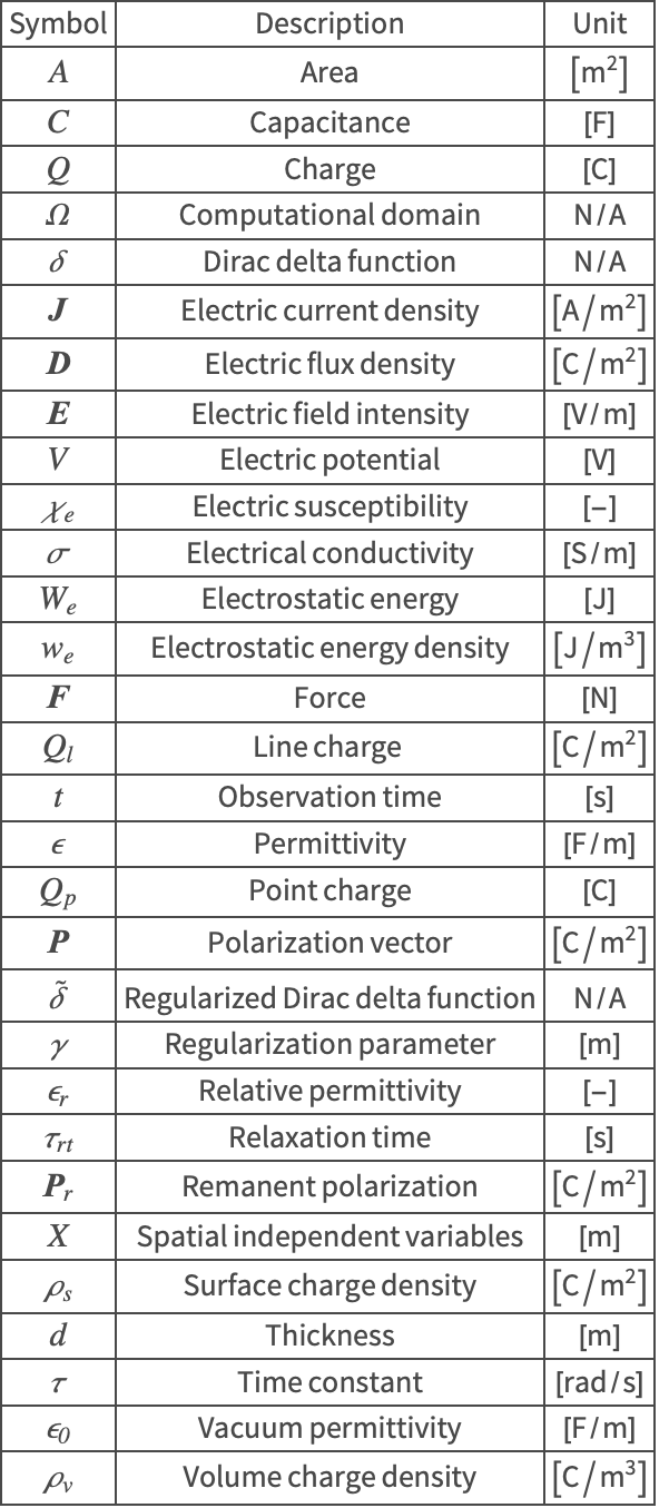
References
1. Bilbao, S. and Hamilton, B. (2017, October). "Directional Source Modeling in Wave-Based Room Acoustics Simulation." In 2017 IEEE Workshop on Applications of Signal Processing to Audio and Acoustics (WASPAA) (pp. 121–125). IEEE.
2. Cardoso, J. R. (2018). Electromagnetics through the Finite Element Method. Boca Raton: CRC Press.
3. Griffiths, D. J. (2017). Introduction to Electrodynamics (4th ed.). Cambridge University Press.
4. Ida, N. and Bastos, J. P. (2013). Electromagnetics and Calculation of Fields. Springer Science & Business Media.
5. Küpfmüller, K. (1968). Einführung in die theoretische Elektrotechnik. Springer.
6. Loucas, A. (2023). "Optimization of Lithium Niobate Electro-optical Modulators" (Master's thesis). Stevens Institute of Technology, New Jersey, NJ.
7. Sadiku, M. N. O. (2011). Elements of Electromagnetics (5th ed.). Oxford University Press.
8. Peskin, C. S. (2002). "The Immersed Boundary Method." Acta Numerica, 11, pp. 479–517.