Spherical Capacitor
Introduction
The following tutorial presents an electrostatic application. This example looks at a spherical capacitor formed of a solid conductor sphere, marked with 1 in the figure, and a hollow spherical conductor shell, marked with 3 in the figure, where the region between the conductors is a dielectric material, marked with 2 in the figure. The aim is to reproduce an electric potential distribution using the finite element method and compare the result to an analytical solution of the capacitance. The following figure shows the geometry of the capacitor in 3D, where the different colors represent the material of each region.

Typically, a 3D electrostatic equation is used to create a partial differential equation model for a 3D capacitor. Since the geometry and the boundary conditions, in this case, are rotationally symmetric about any axis, including the ![]() axis, a 2D axisymmetric electrostatic equation can be used to model the capacitor. An axisymmetric model has the advantage that the computational cost in both time and memory is much less than in the case of solving a full 3D model.
axis, a 2D axisymmetric electrostatic equation can be used to model the capacitor. An axisymmetric model has the advantage that the computational cost in both time and memory is much less than in the case of solving a full 3D model.
Needs["NDSolve`FEM`"]Electrostatic Equation
Electrostatics can be modeled with a Poisson equation. The 2D axisymmetric Poisson equation is given as:
where ![]() is the electric potential in
is the electric potential in ![]() ,
, ![]() is the absolute permittivity in
is the absolute permittivity in ![]() of the material, and
of the material, and ![]() in
in ![]() is the volume charge density.
is the volume charge density.
The axisymmetric Poisson equation uses a truncated cylindrical coordinate system in 2D with independent variables ![]() instead of the cylindrical coordinates
instead of the cylindrical coordinates ![]() . The cylindrical coordinate variable
. The cylindrical coordinate variable ![]() disappears because the system is rotationally symmetric about the
disappears because the system is rotationally symmetric about the ![]() axis. For further reference, see DiffusionPDETerm.
axis. For further reference, see DiffusionPDETerm.
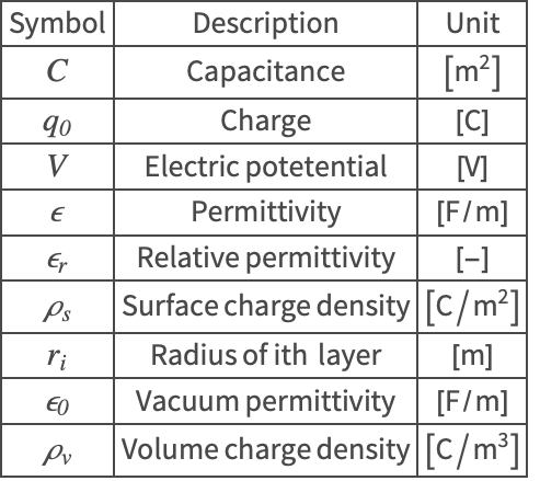
The symbols and corresponding units used throughout this tutorial are summarized in the Nomenclature section.
Model
The model consists of a multilayered ball. The innermost layer, the inner conductor, extends to a radius of ![]() and has a charge of
and has a charge of ![]() . The next layer is a dielectric layer and extends from
. The next layer is a dielectric layer and extends from ![]() to
to ![]() . This is the layer of interest. The outer layer, a second conductor, extends from
. This is the layer of interest. The outer layer, a second conductor, extends from ![]() to
to ![]() . This outer layer is connected to ground and has a potential of
. This outer layer is connected to ground and has a potential of ![]() .
.
Both conductors have different but constant electrostatic conditions. This implies that the potential on each surface is also constant, though different. The goal of this simulation is to compute the distribution of the electric potential in ![]() in the dielectric layer.
in the dielectric layer.
Domain
The domain of the dielectric is an axially symmetric annulus. The external boundaries represent the interfaces between the dielectric and the conductors.
First, the dimensions of the domain are defined, and then an element mesh is created with ToElementMesh.
Subscript[r, 1] = 3 / 1000;
Subscript[r, 2] = 10 / 1000;
Subscript[r, 3] = 12 / 1000;![]() will be used for a three-dimensional visualization.
will be used for a three-dimensional visualization.
a = Annulus[{0, 0}, {Subscript[r, 1], Subscript[r, 2]}, {-π / 2, π / 2}];
mesh = ToElementMesh[a]mesh["Wireframe"]Parameters Setup
Next, the material parameters and the 2D axisymmetric electrostatic equation are set up. These include the relative permittivity ![]() , a dimensionless number and the charge
, a dimensionless number and the charge ![]() .
.
vars = {V[r, z], {r, z}};
pars = <|"RelativePermittivity" -> 3.9|>;Subscript[q, 0] = 6*^-11;The ElectrostaticPDEComponent function can produce the axisymmetric form of the electrostatic equation. To do so, the parameter "RegionSymmetry" is set to "Axisymmetric".
pars["RegionSymmetry"] = "Axisymmetric";op = ElectrostaticPDEComponent[vars, pars];Boundary Conditions
The boundary conditions considered here include both DirichletCondition and NeumannValue. The ElectricPotentialCondition specifies a ground boundary potential of ![]() at the outer boundary of the annulus at
at the outer boundary of the annulus at ![]() . Point element markers will be used here to specify where the ElectricPotentialCondition is applied.
. Point element markers will be used here to specify where the ElectricPotentialCondition is applied.
mesh["PointElementMarkerUnion"]mesh["Wireframe"["MeshElement" -> "PointElements", "MeshElementMarkerStyle" -> Black, "MeshElementStyle" -> {Blue, Yellow, Green, Red, Purple, Purple, Purple, Purple}]]The outer boundary has a point element marker of 3 assigned to it. Because the marker assignment algorithm cannot know what markers are supposed to be assigned at corners, a unique marker is assigned there and thus allows for a choice whether that corner node should be part of the Dirichlet boundary condition or not.
GraphicsRow[{mesh["Wireframe"["MeshElement" -> "PointElements", "MeshElementMarkerStyle" -> Black, "MeshElementStyle" -> {Blue, Yellow, Green, Red, Purple, Purple, Purple, Purple}, PlotRange -> {{-0.001, 0.006}, {0.008, 0.011}}]], mesh["Wireframe"["MeshElement" -> "PointElements", "MeshElementMarkerStyle" -> Black, "MeshElementStyle" -> {Blue, Yellow, Green, Red, Purple, Purple, Purple, Purple}, PlotRange -> {{-0.001, 0.006}, {-0.008, -0.011}}]]}]In the top-left corner is a corner point element marker of 8, and in the bottom-left corner is a point element marker of 7, where the electric potential condition is also to be applied.
Subscript[Γ, p] = ElectricPotentialCondition[ElementMarker == 3 || ElementMarker == 8 || ElementMarker == 7, vars, pars, <|"ElectricPotential" -> 0|>];Point element markers are used for DirichletCondition. For NeumannValue, boundary element markers are to be used. The ElectricFluxDensityValue specifies a surface charge density ![]() in
in ![]() at the boundary of the annulus at
at the boundary of the annulus at ![]() , which represents the charge that has the inner conductor.
, which represents the charge that has the inner conductor.
Subscript[ρ, s] = (Subscript[q, 0]) / 4 / Pi / (Subscript[r, 1] ^ 2);mesh["BoundaryElementMarkerUnion"]mesh["Wireframe"["MeshElement" -> "BoundaryElements", "MeshElementMarkerStyle" -> Black, "MeshElementStyle" -> {Blue, Yellow, Green, Red}]]Subscript[Γ, f] = ElectricFluxDensityValue[ElementMarker == 1, vars, pars, <|"SurfaceChargeDensity" -> Subscript[ρ, s]|>];On a boundary that falls on the symmetry axis, like the ![]() axis in this case, a Neumann 0 value needs to be specified because it is a Symmetry Boundary Condition. As Neumann 0 boundary conditions are the natural default boundary conditions, these can be left out.
axis in this case, a Neumann 0 value needs to be specified because it is a Symmetry Boundary Condition. As Neumann 0 boundary conditions are the natural default boundary conditions, these can be left out.
Model Evaluation
Compute the numeric solution of the PDE with NDSolveValue.
Vfun = NDSolveValue[{op == Subscript[Γ, f], Subscript[Γ, p]}, V, {r, z}∈ mesh]Visualization
DensityPlot[Vfun[r, z], {r, z}∈mesh, ...]Plot[Vfun[r, 0], {r, Subscript[r, 1], Subscript[r, 2]}, PlotRange -> All]To visualize the full 3D solution from the axisymmetric model, one approach is to apply the interpolating function to create a 3D representation of the data. Specifically, a revolution plot of the data can be generated. Using RegionPlot3D, a plot can be created that shows the three-dimensional region where pred is the equation of a sphere with radius ![]() , and a color function is specified to map from the 3D data points to the 2D solution function.
, and a color function is specified to map from the 3D data points to the 2D solution function.
colorFunction = Function[{x, y, z}, Which[x ^ 2 + y ^ 2 + z ^ 2 ≤ Subscript[r, 1]^2, ColorData["BlueGreenYellow", 1], x ^ 2 + y ^ 2 + z ^ 2 >= Subscript[r, 2]^2, ColorData["BlueGreenYellow", 0], True, ColorData[{"BlueGreenYellow", MinMax[Vfun["ValuesOnGrid"]]}][Vfun[Sqrt[x^2 + y^2], z]]]];
Legended[RegionPlot3D[x ^ 2 + y ^ 2 + z ^ 2 ≤ Subscript[r, 3]^2 && 0 ≤ PlanarAngle[{0, 0} -> {{Subscript[r, 3], 0}, {x, y}}] ≤ (4 π/3), {x, -Subscript[r, 3], Subscript[r, 3]}, {y, -Subscript[r, 3], Subscript[r, 3]}, {z, -Subscript[r, 3], Subscript[r, 3]}, ColorFunction -> colorFunction, ...], BarLegend[...]]
Verification
The definition of a capacitance ![]() is given as
is given as
where ![]() is the charge that has the inner conductor sphere and
is the charge that has the inner conductor sphere and ![]() is the potential difference between the conductors.
is the potential difference between the conductors.
For a spherical capacitor, the capacitance is
where ![]() is the relative permittivity of the dielectric layer, which is delimited by the radius
is the relative permittivity of the dielectric layer, which is delimited by the radius ![]() and
and ![]() .
.
See [Hayt & Buck, 2012] for further reference. Alternative methods to compute the capacitance can be found in the Capacitance section of the electrostatics monograph.
c = (Subscript[q, 0]/(Vfun[Subscript[r, 1], 0] - Vfun[Subscript[r, 2], 0]))ϵr = PDEModels`DefaultModelParameters[vars, pars, "Electrostatics"]["RelativePermittivity"];
ϵ0 = PDEModels`DefaultModelParameters[vars, pars, "Electrostatics"]["VacuumPermittivity"];cAnalytic = (4 π ϵ0 * ϵr/(1/Subscript[r, 1]) - (1/Subscript[r, 2]))100 * (Abs[c - cAnalytic]/cAnalytic)Another way to verify the 2D axisymmetric model is to compare it with a full 3D model.
mesh3D = ToElementMesh[RegionDifference[Ball[{0, 0, 0}, Subscript[r, 2]], Ball[{0, 0, 0}, Subscript[r, 1]]]];solution3D = NDSolveValue[{ElectrostaticPDEComponent[{V[x, y, z], {x, y, z}}, <|"RelativePermittivity" -> ϵr|>] == ElectricFluxDensityValue[ElementMarker == 2, {V[x, y, z], {x, y, z}}, <||>, <|"SurfaceChargeDensity" -> Subscript[ρ, s]|>] , ElectricPotentialCondition[ElementMarker == 1, {V[x, y, z], {x, y, z}}, <||>, <|"ElectricPotential" -> 0|>]}, V, {x, y, z} ∈ mesh3D];Plot[Abs[(solution3D[x, 0, 0] - Vfun[x, 0]) / Vfun[x, 0]], {x, Subscript[r, 1], Subscript[r, 2]}]The graph shows that the 2D axisymmetric model matches the full 3D model.
Nomenclature
References
1. Hayt, W. H. and Buck, J. A. (2019). Engineering Electromagnetics. McGraw-Hill Education.