Electric Currents
| Contents | Secondary Quantities |
| Introduction | Boundary Conditions in Electric Currents |
| Overview Example | Nomenclature |
| Equations | References |
Contents
Introduction
This monograph uses partial differential equations to model and analyze electric fields, electric potentials and current distributions. The models presented here consider neither magnetic effects nor electromagnetic radiation.
Magnetic phenomena are considered in the Magnetostatics for Permanent Magnets and the Quasistatic Magnetic Fields monographs.
In this monograph, the focus is on the electric current continuity equation and its main purpose: to compute an electric potential. The equation is mainly used when addressing static and low-frequency device simulations, where magnetic fields and inductive effects can be neglected. This is important: the equation can not be used if magnetic and inductive effects cannot be neglected. One of the key points in this monograph will be to present techniques to establish if the electric current continuity equation can be made use of in a particular scenario.
For the current continuity equation to be valid, both the wavelength ![]() and the skin depth
and the skin depth ![]() must be much larger than the characteristic length
must be much larger than the characteristic length ![]() of the electric device:
of the electric device:
First, consider the wavelength criterion. If the wavelength of an electromagnetic wave is much larger than the characteristic size of the object, ![]() , it means that the time required for the associated electromagnetic wave to propagate at velocity
, it means that the time required for the associated electromagnetic wave to propagate at velocity ![]() over the object size
over the object size ![]() is short compared to the simulation time of interest. Thus, in a low-frequency regime with sufficiently slow time variations, the effects of electromagnetic waves are negligible.
is short compared to the simulation time of interest. Thus, in a low-frequency regime with sufficiently slow time variations, the effects of electromagnetic waves are negligible.
The second criterion that needs to be examined is the skin depth. The skin depth ![]() in [
in [![]() ] is a measure of the depth to which an electromagnetic wave can penetrate a object. The skin effect states that the field intensity depth in a conductor decreases with increasing frequency. For example, the skin depth of copper at 60 [
] is a measure of the depth to which an electromagnetic wave can penetrate a object. The skin effect states that the field intensity depth in a conductor decreases with increasing frequency. For example, the skin depth of copper at 60 [![]() ] is about 8.5 [
] is about 8.5 [![]() ]. This means that in a standard 2.5 [
]. This means that in a standard 2.5 [![]() ] copper wire, the entire cross section of the wire is utilized for an alternating current flow. At higher frequencies, the skin depth becomes much less, and the alternating current flow becomes more and more confined to the surface of the wire. For example, at 2.4 [
] copper wire, the entire cross section of the wire is utilized for an alternating current flow. At higher frequencies, the skin depth becomes much less, and the alternating current flow becomes more and more confined to the surface of the wire. For example, at 2.4 [![]() ], the skin depth in copper is about 1.33 [
], the skin depth in copper is about 1.33 [![]() ]. This effect cannot be modeled with the current continuity equation, so it is essential to ensure that whatever is modeled is not affected by the skin effect.
]. This effect cannot be modeled with the current continuity equation, so it is essential to ensure that whatever is modeled is not affected by the skin effect.
PDEModels`SkinDepth[<|"ElectricalConductivity" -> Quantity[5.998 * 10 ^ 7, "Siemens" / "Meters"], "RelativePermeability" -> 1, "ScaleUnits" -> {"Meters" -> "Millimeters"}, "Quantities" -> True|>, Quantity[60, "Hertz"]]PDEModels`SkinDepth[<|"ElectricalConductivity" -> Quantity[5.998 * 10 ^ 7, "Siemens" / "Meters"], "RelativePermeability" -> 1, "ScaleUnits" -> {"Meters" -> "Micrometers"}, "Quantities" -> True|>, Quantity[2.4, "Gigahertz"]]The skin effect is illustrated in the following figure.

Distribution of current shown in a cross section of a cylindrical conductor. For alternating currents, the current density decreases exponentially from the surface toward the center. The skin depth, ![]() , is defined as the depth at which the current density is just 1/e of the value at the conductor surface.
, is defined as the depth at which the current density is just 1/e of the value at the conductor surface.
More details about the skin effect can be found in the Electromagnetic overview.
The main equation used in this monograph is the electric current continuity equation, given by:
where ![]() [
[![]() ] is the electric current density,
] is the electric current density, ![]() [
[![]() ] is the volume charge density, and
] is the volume charge density, and ![]() is the time variable in [
is the time variable in [![]() ].
].
The current continuity equation is used to model direct currents (DC), general time-varying currents and alternating currents (AC) in conductive and capacitive materials. This equation, once expanded a bit further, will solve for the scalar electric potential ![]() [
[![]() ].
].
An alternative equation that can model static electric fields is the electrostatics equation, discussed in the Electrostatics monograph. Both the electrostatic equation and the current continuity equation solve for the electric potential ![]() and are directly related through the charges that are in a conductive or capacitive media, like electrons. However, each equation models a different phenomenon.
and are directly related through the charges that are in a conductive or capacitive media, like electrons. However, each equation models a different phenomenon.
Modeling electromagnetic devices with partial differential equations (PDEs) is not the only way to model electromagnetic devices. Other techniques include setting up ordinary differential equations (ODEs). This approach is followed by the Wolfram System Modeler. Roughly speaking, the system modeler approach is more suitable for large systems of electromagnetic devices interacting, while the partial differential equation approach is more suitable for a fine-grained analysis of a specific device. In some cases, it is beneficial to use a combination of the two approaches.
The approach taken here is that in the introductory section a capacitor is used to introduce various electromagnetic analysis types and the functionality available. This will be followed by a more theoretical explanation of the underlying ideas and concepts. The theoretical background is much easier to understand once an intuition for the various analysis types exists. After that, the available boundary conditions are discussed.
The goal of this electric device analysis is to find the potential distribution ![]() under specific constraints. A subsequent step then finds secondary fields, such as the electric field intensity
under specific constraints. A subsequent step then finds secondary fields, such as the electric field intensity ![]() [
[![]() ], and values such as the resistance
], and values such as the resistance ![]() . The analysis and interpretation of these physical quantities are useful to create a better quality engineering design of the device under consideration.
. The analysis and interpretation of these physical quantities are useful to create a better quality engineering design of the device under consideration.
The modelng process as such results in a system of partial differential equations (PDEs) that can be solved with NDSolve and ParametricNDSolve.
Extended application examples of electromagnetic modeling can be found in the Model Collection.
The electromagnetic device analysis is typically done in stages. First, for the object to be analyzed, a geometric model needs to be created. The geometric model is typically created within a computer-aided design (CAD) process. CAD models can either be imported or created in product. To import geometries, common file formats like DXF, STL or STEP are supported. These geometries can be imported with Import. The alternative is to create the geometrical models in product, for example, by using OpenCascadeLink.
Once the geometric model is made available, some thought needs to be put into what type of analysis is to be performed. Currently supported analysis types are static analysis, time dependent analysis, frequency response analysis and parametric analysis. The next step is the setup of boundary conditions and constraints. Materials to be used further specify the PDE model. Once the PDE model is fully specified, the subsequent finite element analysis will then compute the desired quantities of the device under investigation. These quantities are then post-processed, either by visualizing them or some derived quantities are computed. This tutorial shows the necessary steps for everything except the CAD model generation.
Electromagnetic devices are typically three-dimensional objects. Special cases exist that result in simplified 2D models. In fact, 2D models have been known to solve 90% of the important problems in electrical engineering [Cardoso, 2018].
The symbols and corresponding units used throughout this tutorial are summarized in the Nomenclature section.
Overview Example
To illustrate the usage of the finite element method in electromagnetics, it is instructive to present a simple example and give an overview of the setup, various analysis types and post-processing steps possible.
Needs["NDSolve`FEM`"]
$HistoryLength = 0;
In this overview example, the workflow of setting up an electric PDE model is introduced. To keep things simple, a fairly simple capacitor is modeled. The capacitor is a well-understood device, demonstrating how to extract different electric properties using various analysis types. A stationary current analysis, a time dependent analysis, a frequency analysis and a parametric analysis will be covered.
In each analysis, the skin depth, denoted as ![]() , will be computed and compared with the characteristic length of the capacitor,
, will be computed and compared with the characteristic length of the capacitor, ![]() . Furthermore, the absolute magnitude of current flow through the capacitor is assumed to be small, implying negligible magnetic fields.
. Furthermore, the absolute magnitude of current flow through the capacitor is assumed to be small, implying negligible magnetic fields.
Consider the following setup with a 3D circular parallel capacitor, composed of two conductive plates with a dielectric in between.

Depiction of a 3D capacitor and the cross section of the dielectric region, in blue.
It is sufficient to model the dielectric region, shown in blue, only.
Creating an electromagnetics model always comprises the same steps:
Geometry
When modeling a capacitor device, there are two possible approaches. One is to consider the device and the surrounding volume. This approach allows for the simulation of the field that appears at the edge of the plates and extends away from the device into the surrounding volume, known as the fringing field. The second approach, used here, considers only the dielectric region. This has the advantage of requiring a smaller geometry to be modeled, resulting in a mesh with fewer elements. Consequently, this approach leads to a shorter runtime compared to the full domain simulation.
Note that in both cases the metal contacts need not be simulated, as the regions of the conductive plates will have the same potential everywhere and can thus be treated as boundaries rather than volume regions.

On the left: A simulation domain of a 2D capacitor and its surrounding volume. To the right: A simulation domain consisting of just the dielectric of a 2D capacitor. In both simulation domains, the conductive plate regions have been removed.
r0 = 0.01;
h = 0.001;L = 2 * r0;Ω = Cylinder[{{0, 0, 0}, {0, 0, h}}, r0];Region[Ω]One thing to keep in mind is the scale used in the geometric model. If the length of the boundary mesh is, for example, in units of meters, then the material parameters will need to be specified in consistent units.
More information on generating or importing 3D geometric models can be found in the Using OpenCascadeLink tutorial.
Material Parameters
The next step is to assign material parameters. Generally, all parameters for an electromagnetics model are collected in an Association pars that includes the necessary parameter values.
The default vacuum permittivity value ![]() [
[![]() ] is used throughout the whole monograph. The "VacuumPermittivity" parameter can also be specified if the constant should have a different value, like 1, to scale the equation.
] is used throughout the whole monograph. The "VacuumPermittivity" parameter can also be specified if the constant should have a different value, like 1, to scale the equation.
In this model, the dielectric of the capacitor will have a relative permittivity ![]() of
of ![]() and an electrical conductivity
and an electrical conductivity ![]() [
[![]() ] of
] of ![]() . These values are just representing a general dielectric material.
. These values are just representing a general dielectric material.
pars = <|"RelativePermittivity" -> 2, "ElectricalConductivity" -> 1*^-8|>;A more convenient way to do material parameter setup is to select a material from an Entity. A convenient way to get to an Entity is to make use of the free-form input.
<|"Material" -> Entity["Element", "Copper"]|>;<|"Material" -> Entity["Element", "Copper"]|>;It is possible to inspect these enriched model parameters.
PDEModels`DefaultModelParameters[{V[x, y, z], {x, y, z}}, <|"Material" -> Entity["Element", "Copper"]|>, "ElectricCurrents"]In the current version of the Wolfram Language, specifying a material Entity works for cases where an electrical conductivity ![]() is used. Values for
is used. Values for ![]() and
and ![]() are currently not available in the material entities.
are currently not available in the material entities.
Material parameters can be given as Quantity objects. Should a material not be available or different units be needed, then the material properties can be added by specifying parameters like "RelativePermittivity" directly.
The full list of properties and their names that can be specified are compiled on the reference pages of ElectricCurrentPDEComponent.
Geometries consisting of several materials can also be used, and an example of such a use case is presented in the section on multiple materials of electric currents.
Units
Should the units of the geometry be different from the material units, then the material units can be scaled. Geometries that are imported from a STEP file will often have units of millimeters.
<|"Material" -> Entity["Element", "Copper"], "ScaleUnits" -> {"Meters" -> "Millimeters"}|>;Internally, all material data units are converted to "SIBase" units. As a consequence, the default unit of length is "Meters". If the units of the geometry are also in meters, then nothing needs to be changed. If the units of the geometry are not in meters, then either the PDE and material properties need to be scaled to the units of the geometry or the geometry needs to be scaled to "Meters". To scale the units of the PDE and material parameters, the parameter "ScaleUnits" can be given. If not explicitly stated otherwise, examples in this tutorial use the default "SIBase" units.
More information about units used in PDEModels can be found in the PDEModels Best Practice tutorial.
Boundary Conditions
Boundary conditions must be defined at physical boundaries to fully specify the problem. In essence, this is done by applying a DirichletCondition or NeumannValue at the boundaries, respectively. Various boundary conditions can be used and will be discussed in more detail in the section Boundary conditions in electric currents. For the purpose of this overview, an electric potential condition and a current density boundary condition will be sufficient. In this case, the device will be charged by applying an electric current though one of the plates.
The purpose of this section is to establish the positions where the boundary conditions are to be applied.
A way to find the positions where the boundary conditions are applied is to visualize them together with the outline geometry defined previously in the geometry section. A current density boundary condition will be applied at the upper plate and an electric potential condition at the lower plate.
upperPlate = z == h;Show[Graphics3D[{Opacity[0.2], Ω}, Boxed -> False], ...]The same technique can be applied at the lower plate.
lowerPlate = z == 0;contour = (x ^ 2 + y ^ 2 == r0 ^ 2) && (0 < z < h);
Show[Graphics3D[{Opacity[0.2], Ω}, Boxed -> False], ...]On the side of the dielectric, an electric insulating condition is applied. This boundary condition means that no electric current flows into the boundary, which is equivalent to a zero NeumannValue. A zero NeumannValue boundary condition is the default boundary condition if nothing else is specified, so this boundary condition can be omitted.
For more complicated geometries, a different technique to specify boundary condition predicates may be more appropriate and is shown in the Spherical Capacitor application example.
Mesh Generation
To perform a finite element analysis, the geometric region needs to be discretized into a mesh.
mesh = ToElementMesh[Ω]More information about the mesh generation process can be found in the ElementMesh generation tutorial. Another option is to import a mesh. Some common mesh file formats can be imported with the help of the FEMAddOns.
Stationary Current Analysis
The first analysis examined is a stationary current analysis, where "stationary" implies no time variation. In this analysis, the primary objective is to determine the electric potential distribution ![]() and, as a secondary derived quantity, the steady current flow
and, as a secondary derived quantity, the steady current flow ![]() [
[![]() ] inside the device. By conducting a stationary current analysis, one can extract the resistance
] inside the device. By conducting a stationary current analysis, one can extract the resistance ![]() of the system.
of the system.
In a stationary analysis, in the limit where the frequency goes to zero, the skin depth goes to infinity. So, the criterion ![]() is satisfied, and the current continuity equation can be used.
is satisfied, and the current continuity equation can be used.
In the case of steady currents, a steady analysis in effect solves the static form of the current continuity equation:
where the time derivative term ![]() has become zero.
has become zero.
Applying Ohm's law to the stationary current continuity equation yields the following equation:
where the dependent variable is the electric potential ![]() , which varies with position
, which varies with position ![]() , and
, and ![]() [
[![]() ] is the electrical conductivity. This equation is the potential version of the current continuity equation and is the equation provided by the function ElectricCurrentPDEComponent.
] is the electrical conductivity. This equation is the potential version of the current continuity equation and is the equation provided by the function ElectricCurrentPDEComponent.
This equation has great similarity with the electrostatic equation (![]() ) provided through ElectrostaticPDEComponent, where electric permittivity
) provided through ElectrostaticPDEComponent, where electric permittivity ![]() is the material constant considered. Note, however, that each of the equations describes a different physical phenomenon, and they are used in different scenarios: The electrostatic equation models electric fields with no currents associated. The current equation models electric fields associated with a current, and this is a reason why this is more suitable for modeling conductors. In contrast, the electrostatic equation is more suitable for modeling dielectric materials.
is the material constant considered. Note, however, that each of the equations describes a different physical phenomenon, and they are used in different scenarios: The electrostatic equation models electric fields with no currents associated. The current equation models electric fields associated with a current, and this is a reason why this is more suitable for modeling conductors. In contrast, the electrostatic equation is more suitable for modeling dielectric materials.
In the following example, however, the analysis treats a dielectric, typically an insulator, as if it were a conductor. The electrical conductivity ![]() of the material is used, which has a value of
of the material is used, which has a value of ![]() [
[![]() ].
].
Perfect insulators are the only materials that have an electrical conductivity of zero; therefore, one cannot model perfect insulators with the current continuity equation.
Treating the dielectric as a conductor will allow you to compute the resistance of the dielectric.
vars = {V[x, y, z], {x, y, z}};op = ElectricCurrentPDEComponent[vars, pars]To charge the device, the capacitor will be fed by applying a normal current density value to one of the plates.
I0 = 0.1*^-6;
Subscript[Γ, current] = ElectricCurrentDensityValue[upperPlate, vars, pars, <|"Current" -> I0|>]
The current of ![]() [
[![]() ] that flows through the upper plate is automatically divided by the area of the surface boundary when calling ElectricCurrentDensityValue.
] that flows through the upper plate is automatically divided by the area of the surface boundary when calling ElectricCurrentDensityValue.
The lower plate will be grounded.
Subscript[Γ, ground] = ElectricPotentialCondition[lowerPlate, vars, pars]These two boundary conditions generate a potential difference between the plates.
Vfun = NDSolveValue[{op == Subscript[Γ, current], Subscript[Γ, ground]}, V, {x, y, z}∈mesh]The result is an InterpolatingFunction object, which gives the electric potential distribution ![]() .
.
More information about the solution process and its options can be found in the NDSolve Options for Finite Elements tutorial.
Post-processing
The primary solution of the electrostatics PDE model is the electric potential.
DensityPlot[Vfun[x, 0, z], {x, -0.01, 0.01}, {z, 0, 0.001}, ...]Also of interest is the electric field intensity ![]() [
[![]() ].
].
Efield = -Grad[Vfun[x, y, z], {x, y, z}]For a three-dimensional model, the function Grad returns a list of three InterpolatingFunction instances with the three independent variables ![]() ,
, ![]() and
and ![]() each.
each.
Efield /. {x -> 0, y -> 0, z -> 0}Various components of the electric field can be accessed by using Part.
Efield[[3]]To compute the resistance ![]() , the values needed are the voltage at the upper plate and the current flowing through the capacitor:
, the values needed are the voltage at the upper plate and the current flowing through the capacitor:
The resistance can be computed with the use of the function ElectricCurrentImpedance.
R0 = PDEModels`ElectricCurrentImpedance[vars, pars, <|"Voltage" -> Vfun, "Current" -> I0|>, mesh, upperPlate]The way this function works is by computing the voltage drop ![]() across the device and then dividing by the current density at that boundary
across the device and then dividing by the current density at that boundary ![]() [
[![]() ]. To get
]. To get ![]() , the function computes the average voltage at the upper plate boundary. In other words, it integrates the voltage Vfun obtained from the model and divides the result by the area of the same boundary.
, the function computes the average voltage at the upper plate boundary. In other words, it integrates the voltage Vfun obtained from the model and divides the result by the area of the same boundary.
Specific details about computations of resistance or impedance values are explained in the Resistance and impedance section. For now, it suffices to know that an impedance is a generalization of a resistance.
Time-Dependent Analysis
A time-dependent analysis in effect solves the transient current continuity equation:
Applying Gauss's law and Ohm's law to the transient current continuity equation yields the following equation:
where ![]() [
[![]() ] is the vacuum permittivity and
] is the vacuum permittivity and ![]() is the unitless relative permittivity. A detailed derivation is provided in the General time-dependent currents section.
is the unitless relative permittivity. A detailed derivation is provided in the General time-dependent currents section.
The transient current continuity equation considers both dielectric (![]() ) and conductive (
) and conductive (![]() ) properties of a material.
) properties of a material.
ElectricCurrentPDEComponent[{V[t, x, y, z], t, {x, y, z}}, <|"ElectricalConductivity" -> σ, "RelativePermittivity" -> Subscript[ϵ, 𝓇], "VacuumPermittivity" -> Subscript[ϵ, 0]|>]Most transient PDEs are characterized by having a single time derivative of the dependent variable term. In the case of the above equation, however, the time derivative term is not independent of a spatial derivative. This can be best seen when the equation is activated.
Activate[ElectricCurrentPDEComponent[{V[t, x, y, z], t, {x, y, z}}, <|"ElectricalConductivity" -> σ, "RelativePermittivity" -> Subscript[ϵ, 𝓇], "VacuumPermittivity" -> Subscript[ϵ, 0]|>]]Before making use of the ElectricCurrentPDEComponent to solve the time dependent equation, a different approach is shown first. A capacitor can be modeled as an ![]() device, the time-dependent behavior of the capacitor can be reproduced without actually solving Eqn. 1. According to literature [Agarwal & Lang, 2018], for an
device, the time-dependent behavior of the capacitor can be reproduced without actually solving Eqn. 1. According to literature [Agarwal & Lang, 2018], for an ![]() device, the current
device, the current ![]() is given by:
is given by:
where ![]() is the time constant
is the time constant ![]() [
[![]() ]. So all that is needed are the resistance and capacitance values of the device.
]. So all that is needed are the resistance and capacitance values of the device.
The resistance value of the capacitor was calculated above.
The capacitance value of the capacitor can be obtained by performing an electrostatics analysis. Such analysis is shown in the overview example of the Electrostatics monograph, where the capacitance value of this same capacitor was calculated.
C0 = 5.52757*^-12;The resistance value is obtained from a stationary electric current analysis, similar to what was done in the stationary section.
R0 = 3.20364430*^8;
tau = C0 * R0I0 = 0.1*^-6;Plot[R0 * I0 * (1 - Exp[-t / tau]), {t, 0, .010}, AxesLabel -> {"t [s]", "V(t) [V]"}, ...]From the plot, it is observed that for large ![]() , the voltage of the capacitor reaches its final value given by
, the voltage of the capacitor reaches its final value given by ![]() [
[![]() ] and that at
] and that at ![]() [
[![]() ], the function reaches
], the function reaches ![]() of its final value.
of its final value.
The plot's increase from ![]() to
to ![]() is characterized by the time constant
is characterized by the time constant ![]() ; in fact, the constant
; in fact, the constant ![]() determines how rapidly the device reaches its stationary behavior.
determines how rapidly the device reaches its stationary behavior.
vars = {V[t, x, y, z], t, {x, y, z}};pars = <|"RelativePermittivity" -> 2, "ElectricalConductivity" -> 1*^-8|>;op = ElectricCurrentPDEComponent[vars, pars]Subscript[Γ, current] = ElectricCurrentDensityValue[upperPlate, vars, pars, <|"Current" -> I0|>]Subscript[Γ, ground] = ElectricPotentialCondition[lowerPlate, vars, pars]For time dependent PDE, additionally to the boundary conditions an initial condition has to be specified. This sets the initial value of the dependent variable at the beginning of the time integration. Specifying a value of 0 means that the system starts at rest.
ic = V[0, x, y, z] == 0;pde = {op == Subscript[Γ, current], ic, Subscript[Γ, ground]};The equation can then be solve by NDSolve. In order to do so an option needs to be specified that makes use of a special parser that can handle the mixed time and space derivatives.
tEnd = 0.01;
Vfun = NDSolveValue[pde, V, {t, 0, tEnd}, {x, y, z}∈Ω, Method -> {"PDEDiscretization" -> {"MethodOfLines", "SpatialDiscretization" -> {"FiniteElement", "Parser" -> "Version14"}}}]Vfun[tEnd, 0, 0, h]v0List = (FEMNBoundaryIntegrate[Vfun[#, x, y, z], {x, y, z}, Vfun["ElementMesh"], upperPlate]& /@ Range[0, tEnd, tEnd / 100]) / FEMNBoundaryIntegrate[1, {x, y, z}, Vfun["ElementMesh"], upperPlate];
v0vsTList = Partition[Riffle[Range[0, tEnd, tEnd / 100], v0List], 2];Grid[{{ListLinePlot[v0vsTList], Plot[R0 * I0 * (1 - Exp[-t / tau]), {t, 0, tEnd}]}}]voA = Rest[R0 * I0 * (1 - Exp[-# / tau])& /@ Range[0, tEnd, tEnd / 100]];
ListLinePlot[((Rest[v0List] - voA) / voA) * 100]Frequency Response Analysis
A frequency response analysis gives information about how a specific variable, in this case, the voltage, behaves to a time-varying sinusoidal input such as a alternating current (AC) at a given frequency ![]() [
[![]() ]. Through a frequency analysis, one can extract the impedance
]. Through a frequency analysis, one can extract the impedance ![]() [
[![]() ] of a system.
] of a system.
In the case of electric currents, a frequency response analysis in effect solves the time-harmonic current continuity equation:
where ![]() [
[![]() ] is the angular frequency and
] is the angular frequency and ![]() the imaginary unit.
the imaginary unit.
Applying Gauss's law and Ohm's law to the time-harmonic current continuity equation yields the following equation:
where ![]() [
[![]() ] is the vacuum permittivity and
] is the vacuum permittivity and ![]() is the unitless relative permittivity. This equation can also be generated by ElectricCurrentPDEComponent. This is done by specifying a angular frequency variable
is the unitless relative permittivity. This equation can also be generated by ElectricCurrentPDEComponent. This is done by specifying a angular frequency variable ![]() [
[![]() ].
].
Like the transient current continuity equation, the time-harmonic version also considers the material's dielectric (![]() ) and conductive (
) and conductive (![]() ) properties.
) properties.
The electric potential ![]() shown in Eqn. 2 is the complex-valued amplitude of the following function:
shown in Eqn. 2 is the complex-valued amplitude of the following function:
where ![]() is known as a phasor. The solution in a frequency analysis will always be a complex number. More details about phasors can be found in the Time Harmonic section.
is known as a phasor. The solution in a frequency analysis will always be a complex number. More details about phasors can be found in the Time Harmonic section.
varsf = {V[x, y, z], ω, {x, y, z}};Note that in the variable specification, the dependent variable is free of ![]() as an independent variable, contrary to a time-dependent variable specification.
as an independent variable, contrary to a time-dependent variable specification.
opf = ElectricCurrentPDEComponent[varsf, pars]As a first case, the behavior of the capacitor under a current excitation that is oscillating at ![]() [
[![]() ] will be examined.
] will be examined.
But first, it will be checked if the criterion ![]() is satisfied. For this dielectric material, a relative permeability
is satisfied. For this dielectric material, a relative permeability ![]() of one will be assumed.
of one will be assumed.
skinDepth = PDEModels`SkinDepth[Append[pars, "RelativePermeability" -> 1], 60]//NLskinDepth > LIt can be seen that the criterion ![]() for the frequency analysis is satisfied.
for the frequency analysis is satisfied.
It is further assumed that the absolute magnitude of the current flow is small, which implies negligible magnetic fields and magnetically induced currents.
f0 = 60;
T0 = 1 / f0;
The boundary conditions are the same as the ones used in the stationary analysis.
Subscript[Γ, ground] = ElectricPotentialCondition[lowerPlate, varsf, pars, <|"ElectricPotential" -> 0|>];The ElectricCurrentDensityValue will be used to excite the capacitor with an AC current that oscillates from ![]() to
to ![]() at
at ![]() [
[![]() ] like a cosine wave. To specify a cosine wave, a real-valued
] like a cosine wave. To specify a cosine wave, a real-valued ![]() is specified. The current will be applied at the upper boundary.
is specified. The current will be applied at the upper boundary.
I0 = 0.1*^-6;
Subscript[Γ, current] = ElectricCurrentDensityValue[upperPlate, varsf, pars, <|"Current" -> I0|>];
If the current value ![]() is expressed from the boundary condition in the time domain using the relation
is expressed from the boundary condition in the time domain using the relation ![]() , upon applying Euler's formula, it simplifies to a cosine function:
, upon applying Euler's formula, it simplifies to a cosine function: ![]() .
.
ComplexExpand[i0 * Exp[I ω t]]Re[ComplexExpand[i0 * Exp[I ω t]]]It is observed that the current amplitude specified in the boundary condition effectively behaves like a cosine wave.
VfunHarmonic = NDSolveValue[{(opf /. {ω -> 2 Pi f0}) == Subscript[Γ, current], Subscript[Γ, ground]}, V, {x, y, z}∈mesh]From this solution, the impedance ![]() [
[![]() ] of the device can be obtained in the same manner as the resistance
] of the device can be obtained in the same manner as the resistance ![]() was obtained.
was obtained.
PDEModels`ElectricCurrentImpedance[varsf, pars, <|"Voltage" -> VfunHarmonic, "Current" -> I0|>, mesh, upperPlate]Specifics about the computation of resistance or impedance values are given in the Resistance and impedance section.
Conduction and displacement currents
To compute the total current density ![]() in a frequency or time analysis, one must take into account that
in a frequency or time analysis, one must take into account that ![]() is composed of the sum of a conduction current
is composed of the sum of a conduction current ![]() and a displacement current
and a displacement current ![]() :
:
So, the time-harmonic current continuity equation can also be expressed as:
By rearranging terms of Eqn. 3, the currents are given by the following equations:
These currents are computed from the electric field ![]() , using the same procedure as shown in the stationary analysis.
, using the same procedure as shown in the stationary analysis.
From frequency domain solution to time domain solution
When performing a frequency analysis, it is possible to transform the solution into the time domain with the following equation:
For specific details on how to transform the solution to the time domain, see the time-harmonic section.
In this case, the time behavior of the solution will be analyzed in the range from ![]() to
to ![]() [
[![]() ].
].
Vlist = Table[{t, Re[VfunHarmonic[0, 0, h] * Exp[I ω t] /. {ω -> 2 Pi f0}]}, {t, 0, 3 * T0, T0 / 100}];Ilist = Table[{t, Re[I0 * Exp[I ω t] /. {ω -> 2 Pi f0}]}, {t, 0, 3 * T0, T0 / 100}];ListLinePlot[{Vlist, Ilist}, MultiaxisArrangement -> All]The voltage can be seen in blue and the current in orange, which has a phase shift between the two.
Parametric Analysis
Sometimes one would like to vary a parameter of a PDE model and repetitively solve the same PDE for a variety of values. A convenient way to do so is a parametric analysis.
As an example, a parametric analysis will be combined with a frequency analysis to study the behavior of the voltage on the capacitor upper plate, which is excited with a square wave current of ![]() [
[![]() ] that goes from
] that goes from ![]() to
to ![]() . In other words, the capacitor is turning on and off periodically.
. In other words, the capacitor is turning on and off periodically.
PDEModels`SkinDepth[Append[pars, "RelativePermeability" -> 1], 60] > LIt can be seen that the criterion ![]() for the parametric frequency analysis is still satisfied.
for the parametric frequency analysis is still satisfied.
For linear materials, Fourier analysis can be utilized to determine the voltage arising from non-harmonic periodic inputs, such as a step function. This approach involves solving for each Fourier coefficient of the square wave individually and then superimposing the solutions ![]() using the principle of superposition. At the end, the solutions can be transformed into the time domain
using the principle of superposition. At the end, the solutions can be transformed into the time domain ![]() .
.
The Fourier series of a square wave of frequency ![]() is given by:
is given by:
where ![]() is the constant current value applied at each period of the square wave, and
is the constant current value applied at each period of the square wave, and ![]() is the fundamental angular frequency with a value of
is the fundamental angular frequency with a value of ![]() .
.
Now, if ![]() is defined as
is defined as ![]() , the equation transforms to:
, the equation transforms to:
In this case, instead of summing up to infinity, the sum will be over a finite number of frequencies.
The finite number of frequencies for the sum will be given by a list of frequencies ranging from ![]() to
to ![]() , where
, where ![]() will be the fundamental frequency, which will be set to
will be the fundamental frequency, which will be set to ![]() [
[![]() ].
].
fRange = Table[f0 + f, {f, 0, 200 * f0, 2 * f0}];As in the stationary and frequency analysis, the capacitor will be excited by applying a current at the upper plate. This is done with an electric current density boundary condition at the upper boundary. The value for the boundary should correspond to Eqn. 4.
To solve for each Fourier coefficient, a parametric study is conducted in ![]() , where
, where ![]() is part of the boundary value expression. The results from each parametric study are then summed up to obtain
is part of the boundary value expression. The results from each parametric study are then summed up to obtain ![]() .
.
As in the frequency analysis, if a ElectricCurrentDensityValue is specified with just a current ![]() , it will behave like a cosine wave with a frequency
, it will behave like a cosine wave with a frequency ![]() that oscillates from
that oscillates from ![]() to
to ![]() .
.
To compute the terms of Eqn. 5, the following equation is used:
Subscript[Γ, currentf] = ElectricCurrentDensityValue[upperPlate, varsf, pars, <|"Current" -> (4I0(2 π f0)/ π ω) * I|>];The imaginary unit ![]() is added to get a sine wave behavior instead of a cosine behavior.
is added to get a sine wave behavior instead of a cosine behavior.
ComplexExpand[i0 * I * Exp[I ω t]]Re[ComplexExpand[i0 * I * Exp[I ω t]]]It is observed that the current amplitude specified in the boundary condition effectively behaves like a sine wave.
VfunAC = ParametricNDSolveValue[{opf == Subscript[Γ, currentf], Subscript[Γ, ground]}, V, {x, y, z}∈mesh, {ω}]Vsolutions = Table[VfunAC[ω] /. {ω -> (2 π) f}, {f, fRange}];The purpose of this example is to see the time behavior of the voltage at the upper plate by using a parametric frequency analysis. The next step is to transform the solutions to the time domain using Eqn. 6.
VsolutionsTime = Table[Re[Vsolutions[[i]][0, 0, h] * Exp[I ω t] /. {ω -> 2 Pi fRange[[i]]}], {i, Length[Vsolutions]}, {t, 0, 3 * T0, T0 / 200}];ITime = Table[Re[I0 * (4 / Pi) * ((2Pi f0) / ω) * I * Exp[I ω t] /. {ω -> 2 Pi fRange[[i]]}], {i, Length[Vsolutions]}, {t, 0, 3 * T0, T0 / 200}];tlist = Table[t, {t, 0, 3 * T0, T0 / 200}];As a last step, one needs to sum all the corresponding voltage contributions of each frequency to get the overall voltage ![]() . The same applies to get the current
. The same applies to get the current ![]() .
.
Vtotal = Total[VsolutionsTime];
Itotal = Total[ITime];Vtime = Partition[Riffle[tlist, Vtotal], 2];
Itime = Partition[Riffle[tlist, Itotal], 2];ListLinePlot[{Vtime, Itime}, MultiaxisArrangement -> All, PlotRange -> Full]The orange line in the plot shows the on and off behavior of the capacitor. The blue line shows how the capacitor is charging and discharging in time.
The resolution of both plots can be improved by using more frequencies or by using more points when transforming the solution to the time domain.
Equations
This section gives an introduction to the partial differential equations (PDEs) for modeling electric currents. Electric currents include direct currents (DC), alternating currents (AC) or general time-dependent currents.
The main equation used in this monograph is the electric current continuity equation, given by:
where ![]() [
[![]() ] is the electric current density,
] is the electric current density, ![]() [
[![]() ] is the volume charge density, and
] is the volume charge density, and ![]() [
[![]() ] is the time variable. It is very important to realize that this equation does not consider inductive or magnetic effects. In other words, this equation cannot be used to model inductive or magnetic effects.
] is the time variable. It is very important to realize that this equation does not consider inductive or magnetic effects. In other words, this equation cannot be used to model inductive or magnetic effects.
When deriving the electric current equation from Maxwell's equations, a simplification is made such that the magnetic fields do not affect the current density. This simplification is necessary to avoid solving the full Maxwell's equations, which can be computationally resource intensive. However, it is essential to ensure that the electric current continuity equation remains applicable in the scenario at hand.
The current continuity equation is typically used to model conductors for which Ohm’s law applies. It is not suitable for modeling perfect insulators where the electrical conductivity is zero ![]() .
.
Electric currents can be modeled in two ways:
Both approaches solve a current continuity problem for the scalar electric potential ![]() .
.
In a steady-state analysis, a direct current flow is generated by a difference in the electric potential. This analysis type is based on the electrical conductivity ![]() of the material under consideration.
of the material under consideration.
In a dynamic simulation, if there are sufficiently slow time variations and sufficiently small dimensions, a quasistatic analysis can be performed. This implies that the time required for an electromagnetic wave to propagate at velocity ![]() over the object size
over the object size ![]() is short compared to the time of interest
is short compared to the time of interest ![]() .
.
where the ratio ![]() is the time required for an electromagnetic wave to propagate through a length
is the time required for an electromagnetic wave to propagate through a length ![]() .
.
Eqn. 7 can be reformulated in terms of the wavelength ![]() . In this case, electromagnetic radiation is negligible if the wavelength
. In this case, electromagnetic radiation is negligible if the wavelength ![]() is much larger than the object size
is much larger than the object size ![]() :
:
Both cases are still under the assumption that inductive and magnetic effects are neglected. That means that the skin depth ![]() of the object considered must be large enough compared to the characteristic size
of the object considered must be large enough compared to the characteristic size ![]() of the object:
of the object: ![]() , as otherwise, magnetic effects need to be considered. This approximation is known as the electroquasistatics approximation of Maxwell's equations.
, as otherwise, magnetic effects need to be considered. This approximation is known as the electroquasistatics approximation of Maxwell's equations.
In the electroquasistatic analysis, conductive effects (![]() ) and capacitive effects (
) and capacitive effects (![]() ) are always considered, as a direct consequence of having a material subjected to a time-dependent electric field. Conductive effects relate to the flow of free electrons that generate an electric current, while capacitive effects involve the storage of electrical energy through the interaction of electric fields with the material and its polarization.
) are always considered, as a direct consequence of having a material subjected to a time-dependent electric field. Conductive effects relate to the flow of free electrons that generate an electric current, while capacitive effects involve the storage of electrical energy through the interaction of electric fields with the material and its polarization.
So, if there is any time variation, the total current will be the sum of a conduction current and a displacement current, where the conduction current is associated with the electrical conductivity ![]() and the displacement current is associated with the capacitive effects and the permittivity
and the displacement current is associated with the capacitive effects and the permittivity ![]() .
.
The current continuity equation can be solved for 1D, 1D axisymmetric, 2D, 2D axisymmetric models and 3D models.
In the following sections, a more detailed explanation and a derivation of the equations are given.
From Maxwell's Equations to the Current Continuity Equation
The derivation of the current continuity equation starts from Maxwell's equations.
where ![]() is the gradient operator,
is the gradient operator, ![]() is the dot product and
is the dot product and ![]() is the cross product. All vector-valued quantities are bold.
is the cross product. All vector-valued quantities are bold. ![]() [
[![]() ] and
] and ![]() [
[![]() ] are the electric and magnetic fields' intensity, respectively.
] are the electric and magnetic fields' intensity, respectively. ![]() [
[![]() ] is the electric flux density, and
] is the electric flux density, and ![]() [
[![]() ]
]![]() [
[![]() ] is the magnetic flux density, sometimes also called magnetic induction. Flux density refers to the flow though an area.
] is the magnetic flux density, sometimes also called magnetic induction. Flux density refers to the flow though an area. ![]() [
[![]() ] is the electric current flux density, commonly called electric current density, and
] is the electric current flux density, commonly called electric current density, and ![]() [
[![]() ] is electric charge density, and they represent sources of a magnetic and electric field, respectively. SI units are used throughout the tutorial.
] is electric charge density, and they represent sources of a magnetic and electric field, respectively. SI units are used throughout the tutorial.
Maxwell's equations, with the exception of Gauss's law of magnetism, form the basis to study the behavior of electric currents. Electric currents can be modeled using Maxwell's equations under two different assumptions: under a static or under a electroquasistatic assumption.
For the case of modeling alternating currents (AC) or time-varying currents, an electroquasistatics approximation needs to be made use of. In the electroquasistatics approximation, Maxwell's equations are:
From Faraday's law (Eqn. 8), the magnetic induction term ![]() was neglected, and from the Maxwell–Ampere law (Eqn. 9), the term
was neglected, and from the Maxwell–Ampere law (Eqn. 9), the term ![]() was conserved.
was conserved.
In the electroquasistatics approximation, the induction term ![]() can be neglected because
can be neglected because ![]() and its time variation are negligibly small. On the other hand, in a stationary analysis, it is valid to have
and its time variation are negligibly small. On the other hand, in a stationary analysis, it is valid to have ![]() , because there are no time variations.
, because there are no time variations.
To derive the electric current continuity equation, consider the following generally true vector identity:
The divergence of the curl of any vector field ![]() is always 0. Applying this identity to Maxwell–Ampere's law (Eqn. 10) results in:
is always 0. Applying this identity to Maxwell–Ampere's law (Eqn. 10) results in:
This means that the magnetic field intensity ![]() is not considered in the electroquasistatic motion of charges.
is not considered in the electroquasistatic motion of charges.
Using Gauss's law (Eqn. 11), the following equation is obtained:
This equation is called the charge density continuity equation and forms the basis to model electric currents. The equation states that the time rate of change of the volume charge density, inside the domain, is equal to the net outward current flow that exits the domain.
The stationary, time-independent version of the current continuity equation is:
This equation is suitable to model direct currents (DC).
As the next step, the constitutive relation that relates the electric field ![]() with the current density
with the current density ![]() is applied, and the current continuity equation is rewritten in terms of the electric scalar potential
is applied, and the current continuity equation is rewritten in terms of the electric scalar potential ![]() .
.
The stationary current continuity in terms of ![]() is:
is:
The derivation of the current continuity equation in terms of ![]() will be shown in the subsequent sections.
will be shown in the subsequent sections.
Despite the fact that magnetic effects are not being considered in the model itself, a magnetic field is always generated as a side effect; it just does not affect the charges modeled. So, it is possible to determine ![]() as a secondary quantity once
as a secondary quantity once ![]() and
and ![]() are fully determined by solving the Maxwell–Ampere law (Eqn. 12) and Gauss's law for magnetism
are fully determined by solving the Maxwell–Ampere law (Eqn. 12) and Gauss's law for magnetism ![]() .
.
Ohm's Law
The constitutive relation for the current continuity equation case is Ohm's law. Ohm's law states that in a conductor, the conduction current density is proportional to the electric field applied across the material. This is because the electric field ![]() in the wire represents a force exerted on the free electrons within the material, causing them to move.
in the wire represents a force exerted on the free electrons within the material, causing them to move.

A conductor under an applied ![]() field. The direction of the electric field
field. The direction of the electric field ![]() is opposite to the direction of the flow of electrons.
is opposite to the direction of the flow of electrons.
where ![]() [
[![]() ] is the electrical conductivity.
] is the electrical conductivity.
The conductivity ![]() of a material therefore measures the extent to which electrons in the material respond to an applied field. For any other type of material, where electrons are not the primary carriers, other models are needed.
of a material therefore measures the extent to which electrons in the material respond to an applied field. For any other type of material, where electrons are not the primary carriers, other models are needed.
A more general version of Ohm’s law includes an externally generated current density ![]() [
[![]() ] that is given by:
] that is given by:
![]() does not have an electric field
does not have an electric field ![]() associated with it.
associated with it.
Faraday's law, ![]() , (Eqn. 13) states that
, (Eqn. 13) states that ![]() is curl free and allows the scalar electric potential
is curl free and allows the scalar electric potential ![]() to be derived.
to be derived.
Generally speaking, for fields, the following equation can be deduced:
which states that the curl of the gradient of any scalar function ![]() is zero. Comparing Eqn. 14 with Faraday's law, it can be deduced that
is zero. Comparing Eqn. 14 with Faraday's law, it can be deduced that ![]() can be represented as the gradient of a function
can be represented as the gradient of a function ![]() :
:
The negative sign was placed by convenience and for historical reasons.
Now that Ohm's law and the electric scalar potential have been established, they can be substituted into the current continuity equation to finally get the equations needed.
Stationary Currents or Direct Currents
For steady analysis, a combination of the current continuity equation and Maxwell's equations is used to derive the fundamental equation for direct currents in a material described by Ohm's law.
For direct currents (DC), it holds that the rate of change of the charge density is zero:
So, the current continuity equation takes the following form:
Using Eqn. 15 and Eqn. 16, the current continuity equation becomes:
The dependent variable in this equation is the electric potential ![]() [
[![]() ], which varies with position
], which varies with position ![]() . The equation is made up of a diffusive term
. The equation is made up of a diffusive term ![]() , with the electrical conductivity
, with the electrical conductivity ![]() [
[![]() ] as the diffusion coefficient.
] as the diffusion coefficient.
This equation is used to model direct currents in conductors. Perfectly insulating materials are removed from the simulation domain, and exterior perfectly insulating surfaces are modeled as boundaries.
The current continuity equation can be generalized to include current sources:
The term ![]() [
[![]() ] denotes a volumetric current source within the domain, which can appear on the right-hand side of the equation, and it is explained in the Source Types section.
] denotes a volumetric current source within the domain, which can appear on the right-hand side of the equation, and it is explained in the Source Types section.
Also, one can add an externally generated current density![]() [
[![]() ] to the equation:
] to the equation:
The external current density does not have an electric field associated with it. This additional term is modeled as an additional derivative term ![]() .
.
When direct currents are simulated, magnetic fields are produced as a byproduct. However, since the magnetic field is stationary, it does not generate induced currents. As a result, once the steady currents are known, the magnetic field can be fully determined and computed using ![]() .
.
Dynamic Currents
In the following sections, a general time-dependent current continuity equation and a time-harmonic current continuity equation are derived. This is done by combining the current continuity equation with Gauss's law. The equations in both cases are in terms of the electric potential ![]() .
.
General time-dependent currents
In this case, the current continuity equation maintains its time-derivative term and ![]() is substituted with
is substituted with ![]() according to Gauss's law:
according to Gauss's law:
Reorganizing the equation, the result is:
The electric flux density ![]() is defined as:
is defined as:
which is the constitutive relation between the electric field intensity ![]() and the electric flux density
and the electric flux density ![]() .
. ![]() is the polarization vector in units of [
is the polarization vector in units of [![]() ].
].
Inserting this constitutive relation between ![]() and
and ![]() (Eqn. 17) and Ohm's law (Eqn. 18) into Eqn. 19, the result is:
(Eqn. 17) and Ohm's law (Eqn. 18) into Eqn. 19, the result is:
And finally, by inserting ![]() , the transient current continuity equation is obtained:
, the transient current continuity equation is obtained:
Separating terms, the final and most general version of the current continuity equation is:
The time-dependent current continuity equation consists of two parts. The first term is the time-dependent version of the stationary current continuity equation. The second part is the time derivative of the volume charge density (Eqn. 20) and is similar in spirit to the electrostatic equation with the exception of the time derivative. This is the reason that the parameter names of the current continuity equation are the same as the parameter names of the electrostatic equation.
Next, consider the meaning of these terms. The first term ![]() refers to a conduction current
refers to a conduction current ![]() , and the second term
, and the second term ![]() refers to a displacement current
refers to a displacement current ![]() .
.
The conduction current ![]() is always associated with the electric field through Ohm's law. The conduction current is associated with the movement of free electrons in conducting materials.
is always associated with the electric field through Ohm's law. The conduction current is associated with the movement of free electrons in conducting materials.
The displacement current ![]() itself consists of two parts in a dielectric: an electric field part depending on
itself consists of two parts in a dielectric: an electric field part depending on ![]() and a polarization part depending on
and a polarization part depending on ![]() . A device under consideration is excited by applying a time-varying current or time-varying voltage difference. The electric field component comes from this excitation field and is present in both the material media and in free space surrounding the media. The polarization part is a field produced by the movement of dielectric material bound charges in the excitation field. The name displacement field comes from the fact that
. A device under consideration is excited by applying a time-varying current or time-varying voltage difference. The electric field component comes from this excitation field and is present in both the material media and in free space surrounding the media. The polarization part is a field produced by the movement of dielectric material bound charges in the excitation field. The name displacement field comes from the fact that ![]() and
and ![]() is often called displacement field. In simple terms, the displacement current is a time derivative of the displacement field
is often called displacement field. In simple terms, the displacement current is a time derivative of the displacement field ![]() .
.
Note that in the displacement current ![]() , there is a time derivative inside the divergence operator. In current versions of the Wolfram Language, equations with such a mixed spatial/temporal derivative can be solved by specifying a special option to NDSolve and related functions.
, there is a time derivative inside the divergence operator. In current versions of the Wolfram Language, equations with such a mixed spatial/temporal derivative can be solved by specifying a special option to NDSolve and related functions.
Method -> {"PDEDiscretization" -> {"MethodOfLines", "SpatialDiscretization" -> {"FiniteElement", "Parser" -> "Version14"}}};Since the time-dependent current continuity equation has a conducting term and a dielectric term, the equation can be used to model both conductors and dielectric material. In good conductors, the conduction current will be much larger than the displacement current when subjected to a time-varying field. This means that for good conductors, ![]() , while in good dielectrics, the opposite is true.
, while in good dielectrics, the opposite is true.
Since magnetic fields are not considered in the electric current continuity equation, it is often a fair assumption to make that metal contracts are equipotential. This assumption allows one not to discretize that region and eventually save the computational time to solve the equation in these regions.
In the case of linear materials, where ![]() varies linearly with
varies linearly with ![]() , the polarization can be expressed as
, the polarization can be expressed as ![]() . This is described in the electrostatics monograph. As a consequence, the constitutive relation between
. This is described in the electrostatics monograph. As a consequence, the constitutive relation between ![]() and
and ![]() changes such that
changes such that ![]() and
and ![]() . This transformation is useful since for many materials, polarization data is not available, but the relative permittivity
. This transformation is useful since for many materials, polarization data is not available, but the relative permittivity ![]() is. Concerning the implementation of ElectricCurrentPDEComponent, both formulations can be used.
is. Concerning the implementation of ElectricCurrentPDEComponent, both formulations can be used.
The time-dependent current continuity equation can also be generalized to include a current source ![]() :
:
or with a relative permittivity ![]() formulation:
formulation:
The time-dependent current continuity equation is valid only if the skin depth ![]() is much larger than the characteristic length
is much larger than the characteristic length ![]() of the electric device
of the electric device ![]() .
.
Alternating currents (AC)
In a frequency analysis, time-harmonic currents are modeled. These are currents that vary in a harmonic form, like a sinusoidal form, and are known as alternating currents (AC). The purpose of a frequency analysis is to compute the frequency response of an electric system over a range of frequencies. The frequency analysis of a model is done with ParametricNDSolve.
An electric field or electric potential is referred to as time harmonic if it can be expressed as a sine function with a specific frequency. For a time-harmonic analysis, an electric system is exposed to several harmonic input signals over a range of frequencies, and the performance of the device at frequencies of interest is analyzed.
In response to a harmonic stimulus, the resulting electric potential ![]() can be shown to be time harmonic as well. An electric potential is said to be time harmonic if the potential variation at any spatial position
can be shown to be time harmonic as well. An electric potential is said to be time harmonic if the potential variation at any spatial position ![]() has a sinusoidal time dependence with an angular frequency
has a sinusoidal time dependence with an angular frequency ![]() .
.
A general expression of a harmonic electric potential ![]() is written as:
is written as:
Here ![]() denotes the amplitude at the given position, and
denotes the amplitude at the given position, and ![]() is an initial phase shift at
is an initial phase shift at ![]() .
.
For analytical convenience, the time-harmonic relation (21) is often expressed in complex-valued form, known as both the complex exponential representation (CER) and the phasor equation:
where ![]() is the imaginary unit and the factor
is the imaginary unit and the factor ![]() is equal to
is equal to ![]() .
.
By convention, the phasor is often expressed simply as:
in which it is implicitly interpreted that the real part of the complex-valued expression represents the real function ![]() .
.
The phasor can be understood as a rotating vector ![]() in the complex plane. The following figure illustrates this behavior.
in the complex plane. The following figure illustrates this behavior.

A phasor represented in the complex plane at ![]() and at
and at ![]() .
.
The rotating vector ![]() is known as the complex amplitude function. The amplitude function
is known as the complex amplitude function. The amplitude function ![]() rotates counterclockwise at a speed of the angular frequency
rotates counterclockwise at a speed of the angular frequency ![]() . At any given time
. At any given time ![]() , the projection of
, the projection of ![]() on the real axis represents the transient electric potential
on the real axis represents the transient electric potential ![]() , and the vector length
, and the vector length ![]() corresponds to the local amplitude.
corresponds to the local amplitude.
If the amplitude function and its complex conjugate are expressed as ![]() and
and ![]() , then the local amplitude
, then the local amplitude ![]() can be calculated by:
can be calculated by:
Phasors are applicable only for linear systems, meaning that no material property can depend on the field under study. For nonlinear materials, it is necessary to solve the system in the time domain.
When the phasor equation is inserted in the time-dependent current continuity equation, the equation simplifies to a time-independent current continuity equation. The phasor equation expresses the time-dependent potential as a product of the potential amplitude ![]() with the time factor
with the time factor ![]() .
.
The external current density and the polarization vector can be expressed in the same way with amplitude functions ![]() and
and ![]() and the same time factor
and the same time factor ![]() :
:
The time-dependent current continuity equation is given as:
By inserting (22) and (23) into the time-dependent current continuity (24), the following is obtained:
The gradient ![]() can be rewritten as:
can be rewritten as:
since the ![]() term does not depend on space. This leads to:
term does not depend on space. This leads to:
Next, consider the part of Eqn. 25 that has the first-order time-derivative term and expand it:
Reinserting the expanded term into Eqn. 26 gives:
Factoring out the common terms ![]() and
and ![]() , the equation simplifies to the time-harmonic current continuity equation:
, the equation simplifies to the time-harmonic current continuity equation:
The time-harmonic current continuity equation consists of two parts. The first term is the stationary current continuity equation, and the second part is the frequency version of the time derivative of the volume charge density (![]() ). Note that this part is very similar to the electrostatic equation
). Note that this part is very similar to the electrostatic equation ![]() , with the exception of the
, with the exception of the ![]() term. This is the reason that the parameter names of the current continuity equation are the same as the parameter names of the electrostatic equation.
term. This is the reason that the parameter names of the current continuity equation are the same as the parameter names of the electrostatic equation.
As in the time-dependent current continuity equation, the first term ![]() refers to a conduction current, and the second term
refers to a conduction current, and the second term ![]() refers to a displacement current.
refers to a displacement current.
Since the time-harmonic current continuity equation has a conducting term and a dielectric term, the equation can be used to model both conductors and dielectric material.
This PDE is a time-independent equation. Because it is a time-independent PDE, it can be solved more efficiently compared to the time-dependent current continuity equation used for modeling electric currents in the time domain.
However, in a linear system, a sinusoidal input will yield a sinusoidal output. This property is fundamental for time-harmonic analysis. In contrast, for nonlinear materials, this linearity property does not hold, and therefore harmonic analysis cannot be applied. In the case of nonlinear materials, a full time-dependent simulation is necessary.
In the case of linear materials, the polarization becomes ![]() . This is explained in the electrostatics monograph. This then changes the constitutive relation between
. This is explained in the electrostatics monograph. This then changes the constitutive relation between ![]() and
and ![]() such that
such that ![]() and
and ![]() . This transformation is useful since for many materials, polarization data is not available, but the relative permittivity
. This transformation is useful since for many materials, polarization data is not available, but the relative permittivity ![]() is. Concerning the implementation of ElectricCurrentPDEComponent, both formulations can be used.
is. Concerning the implementation of ElectricCurrentPDEComponent, both formulations can be used.
The time-harmonic current continuity equation can also be generalized to include a current source ![]() :
:
The time-harmonic current continuity equation is valid only if the skin depth ![]() is much larger than the characteristic length
is much larger than the characteristic length ![]() of the electric device
of the electric device ![]() .
.
In the case of non-harmonic periodic inputs, such as current step function ![]() , Fourier analysis can be employed to determine the fields arising.This approach involves solving the time-harmonic current continuity equation for each Fourier coefficient of the non-harmonic periodic input, such as a periodic step function individually, and then constructing the solution by using the principle of superposition.
, Fourier analysis can be employed to determine the fields arising.This approach involves solving the time-harmonic current continuity equation for each Fourier coefficient of the non-harmonic periodic input, such as a periodic step function individually, and then constructing the solution by using the principle of superposition.
The computed solution ![]() can be easily transformed back into time domain using the time-harmonic relation (Eqn. 27).
can be easily transformed back into time domain using the time-harmonic relation (Eqn. 27).
Electric Currents Model Setup
The stationary and the dynamic current continuity equations shown in this section can all be generated by ElectricCurrentPDEComponent.
To make use of this PDE operator, variables vars and parameters pars need to be set up. The following subsections show how to do that for the various cases.
Static electric currents model setup
The static electric current continuity equation is given by:
To specify a PDE model, model variables vars need to be set up. Stationary variables are specified as vars={V[x,y,…],{x,y,…}}, where the dependent variable ![]() is the electric potential in units of [
is the electric potential in units of [![]() ] and the {x,y,…} are the independent spatial variables in units of [
] and the {x,y,…} are the independent spatial variables in units of [![]() ].
].
The following is a list of possible parameters pars that can be specified for a steady current model:
ElectricCurrentPDEComponent[{V[x, y, z], {x, y, z}}, <|"ElectricalConductivity" -> σ * IdentityMatrix[3], "ExternalCurrentSource" -> {Jex[x, y, z], Jey[x, y, z], Jez[x, y, z]}|>]Note that this model definition uses inactive PDE operators. "Numerical Solution of Partial Differential Equations" has several sections that explain the use of inactive operators.
Dynamic electric currents model setup
For a dynamic model, one can either set up a frequency or time-dependent model.
For a both dynamic models, the static electric currents parameters pars can be used:

Additionally, the following parameters, explained in detail in the electrostatic monograph, are available:
The time-dependent electric current continuity equation is given by:
To specify the time-dependent model, variables are specified as vars={V[t,x,y,…],t,{x,y,…}}, where ![]() is the time variable in units of [
is the time variable in units of [![]() ].
].
ElectricCurrentPDEComponent[{V[t, x, y], t, {x, y}}, <|"ElectricalConductivity" -> σ * IdentityMatrix[2], "ExternalCurrentSource" -> {Jex[t, x, y], Jey[t, x, y]}, "VacuumPermittivity" -> Subscript[ϵ, 0], "RelativePermittivity" -> Subscript[ϵ, 𝓇] * IdentityMatrix[2]|>]In the current version of NDSolve, an option needs to be specified to be able to solve mixed time and spacial derivatives.
Method -> {"PDEDiscretization" -> {"MethodOfLines", "SpatialDiscretization" -> {"FiniteElement", "Parser" -> "Version14"}}};The frequency-dependent electric current continuity equation is given by:
To specify a frequency-dependent model, variables are specified as vars={V[x,y,…],ω,{x,y,…}}, where ![]() is the angular frequency. Note that in this case, the angular frequency
is the angular frequency. Note that in this case, the angular frequency ![]() is not an argument of the dependent variable
is not an argument of the dependent variable ![]() .
.
ElectricCurrentPDEComponent[{V[x, y, z], ω, {x, y, z}}, <|"ElectricalConductivity" -> σ * IdentityMatrix[3], "ExternalCurrentSource" -> {Jex[x, y, z], Jey[x, y, z], Jez[x, y, z]}, "VacuumPermittivity" -> Subscript[ϵ, 0], "RelativePermittivity" -> Subscript[ϵ, 𝓇] * IdentityMatrix[3]|>]2D models
When the electric potential ![]() varies only in the
varies only in the ![]() and
and ![]() directions and is constant in the
directions and is constant in the ![]() direction, a 3D model can be modeled as a 2D model in the
direction, a 3D model can be modeled as a 2D model in the ![]() -
-![]() plane.
plane.
This type of symmetry is seen frequently in rotating electric machines, in which the field distribution is repeated in planes parallel to the cross section of the electric machine [Cardoso, 2018].

Conduction in a rectangular plate. In the image on the left, the electric potential ![]() is visualized over the whole domain. The plot shows that the electric potential does not vary with respect to
is visualized over the whole domain. The plot shows that the electric potential does not vary with respect to ![]() , so it is possible to model the domain in the
, so it is possible to model the domain in the ![]() -
-![]() plane. In the image on the right, the difference between the solution at
plane. In the image on the right, the difference between the solution at ![]() and at
and at ![]() is shown, being negligible.
is shown, being negligible.
With this symmetry, the following equation is solved:
where ![]() [
[![]() ] is a thickness variable denoting thickness in the
] is a thickness variable denoting thickness in the ![]() direction.
direction.
ElectricCurrentPDEComponent[{V[x, y], {x, y}}, <|"ElectricalConductivity" -> σ * IdentityMatrix[2], "Thickness" -> d|>]The default value for the thickness is ![]() .
.
1D models
When the electric potential ![]() in a 3D model remains constant along the
in a 3D model remains constant along the ![]() and
and ![]() directions, the model can be simplified to a 1D representation. In this 1D model of electric currents, a cross-sectional area
directions, the model can be simplified to a 1D representation. In this 1D model of electric currents, a cross-sectional area ![]() [
[![]() ], encompassing the
], encompassing the ![]() and
and ![]() directions, is incorporated into the equation:
directions, is incorporated into the equation:
The default value for the cross-sectional area is ![]() .
.
ElectricCurrentPDEComponent[{V[x], {x}}, <|"ElectricalConductivity" -> σ * IdentityMatrix[1], "CrossSectionalArea" -> A|>]Axisymmetric Electric Currents Models
2D axisymmetric
An axisymmetric simulation can be performed when a 3D solid has an axis of revolution. An axisymmetric model uses a truncated cylindrical coordinate system in 2D with independent variables ![]() instead of the cylindrical coordinates
instead of the cylindrical coordinates ![]() . The cylindrical coordinate variable
. The cylindrical coordinate variable ![]() disappears because the system is rotationally symmetric about the
disappears because the system is rotationally symmetric about the ![]() axis.
axis.
The 2D axisymmetric equation for steady currents for linear materials is given as:
An axisymmetric model has the advantage that the computational cost in both time and memory is much less than in the case of solving a full 3D model.
The ElectricCurrentPDEComponent function can produce the axisymmetric form of the stationary current continuity equation. To do so, the parameter "RegionSymmetry" is set to "Axisymmetric".
ElectricCurrentPDEComponent[{V[r, z], {r, z}}, <|"ElectricalConductivity" -> σ * IdentityMatrix[2], "RegionSymmetry" -> "Axisymmetric"|>]A 2D axisymmetric model can also be generated for the frequency- and time-dependent equation variations, and also when using an external current ![]() .
.
ElectricCurrentPDEComponent[{V[r, z], ω, {r, z}}, <|"VacuumPermittivity" -> Subscript[ϵ, 0], "ElectricalConductivity" -> σ * IdentityMatrix[2], "RelativePermittivity" -> Subscript[ϵ, 𝓇] * IdentityMatrix[2], "RegionSymmetry" -> "Axisymmetric"|>]In this case, the electric potential is constant in the ![]() direction, which implies that the electric field is tangential to the
direction, which implies that the electric field is tangential to the ![]() -
-![]() plane. The Spherical Capacitor model shows a 2D axisymmetric model in use.
plane. The Spherical Capacitor model shows a 2D axisymmetric model in use.
1D axisymmetric
In 1D axisymmetric geometries, the electric potential is constant in both the ![]() direction and the
direction and the ![]() direction. The 1D axisymmetric equation for steady currents for linear materials is given as:
direction. The 1D axisymmetric equation for steady currents for linear materials is given as:
where ![]() [
[![]() ] is the thickness variable denoting thickness in the
] is the thickness variable denoting thickness in the ![]() direction.
direction.
ElectricCurrentPDEComponent[{V[r], {r}}, <|"ElectricalConductivity" -> σ * IdentityMatrix[1], "RegionSymmetry" -> "Axisymmetric", "Thickness" -> d|>]Anisotropic Materials
An anisotropic material is a material whose properties, such as mechanical, thermal or electrical, exhibit different behavior in different directions, as opposed to being uniform, isotropic in all directions.
For anisotropic conductors, the electrical conductivity ![]() is a tensor. In the 3D case, the tensor has nine components:
is a tensor. In the 3D case, the tensor has nine components:
where ![]() is the electrical conductivity tensor.
is the electrical conductivity tensor. ![]() and
and ![]() are called the principal conductivity coefficients and off-diagonal conductivity coefficients, respectively.
are called the principal conductivity coefficients and off-diagonal conductivity coefficients, respectively.
ElectricCurrentPDEComponent[{V[x, y], {x, y}}, <|
	"ElectricalConductivity" -> {{Subscript[σ, xx], Subscript[σ, xy]}, {Subscript[σ, yx], Subscript[σ, yy]}}|>]
Multiple Materials
It is common that a device intended for modeling consists of multiple materials. Therefore, it is necessary to model different materials in the simulation domain. To show the process of simulating multimaterial regions, a two-material plate is modeled.
Consider an upper layer of copper connected to a lower layer of iron. The left boundary of the copper layer serves as a potential contact and the lower right boundary of the iron material serves as a ground contact. The current then flows from the upper left to the lower right.

Plate of two different metals. The upper section is made up copper and the lower section of iron.
Lx = Ly = 1;bmesh = ToBoundaryMesh["Coordinates" -> {{-Lx, -Ly}, {Lx, -Ly}, {Lx, 0}, {Lx, Ly}, {-Lx, Ly}, {-Lx, 0}}, "BoundaryElements" -> {LineElement[{{1, 2}, {2, 4}, {4, 5}, {5, 1}, {3, 6}}]}];The use of element markers will be employed here to give the different conductivities to the subdomains.
materials = <|"copper" -> 1, "iron" -> 2|>;mesh = ToElementMesh[bmesh, "RegionMarker" -> {{{0, Ly / 2}, materials["copper"]}, {{0, -Ly / 2}, materials["iron"]}}];vars = {V[x, y], {x, y}};
pars = <|"Material" -> {{ElementMarker == materials["copper"], Entity["Element", "Copper"]}, {True, Entity["Element", "Iron"]}}|>;op = ElectricCurrentPDEComponent[vars, pars];The upper-left corner will be grounded while the lower-right corner will have a potential of one.
Subscript[Γ, potentials] = {ElectricPotentialCondition[x == Lx && -Ly ≤ y ≤ 0, vars, pars], ElectricPotentialCondition[x == -Lx && 0 ≤ y ≤ Ly, vars, pars, <|"ElectricPotential" -> 1|>]};When no "ElectricPotential" value is specified for a ElectricPotentialCondition, it will be set to ground (0) by default.
Vfun = NDSolveValue[{op == 0, Subscript[Γ, potentials]}, V, {x, y}∈mesh];ContourPlot[Vfun[x, y], {x, y}∈ mesh, ...]From the electric potential plot, it is evident that the potential is ![]() continuous across the copper/iron interface.
continuous across the copper/iron interface.
If one wants to compute the electric field intensity ![]() and the current density
and the current density ![]() , one has to take into account that at interfaces between different materials, the fields can be discontinuous. More information about these conditions can be found in the section Interface conditions. Next, examine how to solve this.
, one has to take into account that at interfaces between different materials, the fields can be discontinuous. More information about these conditions can be found in the section Interface conditions. Next, examine how to solve this.
In this example, ![]() and
and ![]() will exhibit a discontinuity at the interface.
will exhibit a discontinuity at the interface.
Efield = -Grad[Vfun[x, y], {x, y}];Plot[Efield[[2]] /. {x -> 0}, {y, -1, 1}]The above plot shows the discontinuity across the material interface running along the axis ![]() . There are values of
. There are values of ![]() and
and ![]() , coming from the left and right, respectively, at the same time.
, coming from the left and right, respectively, at the same time.
What is problematic is that there is no control over what the value is along the interface.
Plot[Efield[[2]] /. {y -> 0}, {x, -1, 1}, PlotRange -> {0, -2.7}]Note that there is no control over what the value of the field at the interface is, which can be seen by the jiggled plot line. When evaluating an InterpolatingFunction at the material interface, it is somewhat random if the value of the one material subregion or the other subregion is given.
To address this issue, use DiscontinuousInterpolatingFunction or EvaluateOnElementMesh. This process will be shown next.
First, the electric potential function ![]() is converted to a DiscontinuousInterpolatingFunction.
is converted to a DiscontinuousInterpolatingFunction.
VfunDIF = DiscontinuousInterpolatingFunction[Vfun] The electric field intensity ![]() is the gradient and will be computed in a second step.
is the gradient and will be computed in a second step.
EfieldDIF = -Grad[VfunDIF[x, y], {x, y}]Plot[EfieldDIF[[2]] /. {x -> 0}, {y, -1, 1}]Plot[EfieldDIF[[2]] /. {y -> 0}, {x, -1, 1}, PlotRange -> {0, -2.7}]EfieldDIF[[2]] /. {x -> 0, y -> 0}Note that the value that is returned at the discontinuity is the value of copper. The behavior of what takes precedence over what can be controlled. DiscontinuousInterpolatingFunction or EvaluateOnElementMesh functions will prioritize a value from one of the subregions. The default is based on the order of material markers.
mesh["MeshElementMarkerUnion"]In this case, the default is to prioritize the copper region over the iron region. To demonstrate the usage of marker prioritization, gradients will be recomputed with a priority favoring the iron region over the copper region.
VfunDIFIron = DiscontinuousInterpolatingFunction[Vfun, "MarkerPriority" -> {2, 1}];
EfieldIronDIF = -Grad[VfunDIFIron[x, y], {x, y}]{EfieldIronDIF[[2]], EfieldDIF[[2]]} /. {x -> 0, y -> 0}With this technique, there is precise control over what happens at the interface—which material subregion has presidency over which other subregion. DiscontinuousInterpolatingFunction is very useful to compute values at the interface between two different materials and then use them in plots or as arguments for further computations.
The same technique can be applied when computing other quantities such as the current density vector ![]() , where
, where ![]() varies continuously across the interface, whereas
varies continuously across the interface, whereas ![]() shows a discontinuity. Next, the current density vector
shows a discontinuity. Next, the current density vector ![]() is computed:
is computed:
The electrical conductivity ![]() is a Piecewise function in this case, resulting in a discontinuity at the material boundary. Use EvaluateOnElementMesh to create the DiscontinuousInterpolatingFunction.
is a Piecewise function in this case, resulting in a discontinuity at the material boundary. Use EvaluateOnElementMesh to create the DiscontinuousInterpolatingFunction.
σ0 = PDEModels`DefaultModelParameters[vars, pars, "ElectricCurrents"]["ElectricalConductivity"];J = Through[EvaluateOnElementMesh[{x, y}, -σ0.EfieldDIF, mesh][x, y]]Show[ContourPlot[Vfun[x, y], {x, y}∈ mesh, ...], VectorPlot[J, {x, y}∈mesh, ...], bmesh["Wireframe"]]From the plot, it can be seen that the current flow ![]() is perpendicular to the contours of
is perpendicular to the contours of ![]() , as expected. At the interface, the current direction of
, as expected. At the interface, the current direction of ![]() is refracted.
is refracted.
Source Types
The current continuity equation can be generalized to include current sources ![]() which are always in units of [
which are always in units of [![]() ]. The source term is often zero, but in some cases it might be necessary to add it to the equation.
]. The source term is often zero, but in some cases it might be necessary to add it to the equation.
The presentation of the various source types follows the same structure used in the Electrostatics monograph. Based on their shape, sources are categorized as volume, line, and point sources. Sources are much less commonly used in electrical current models than in electrostatic models. It is much less clear what a current source physically looks like. Nevertheless, you can set them up. For actual code examples, refer to the electrostatics monograph, where there are examples of a volume charge density, a point charge in 3D or a line charge in 2D.
Volume current source
The source term ![]() [
[![]() ] on the right-hand side of the current continuity equation is used as a source to generate an internal electric field
] on the right-hand side of the current continuity equation is used as a source to generate an internal electric field ![]() , acting as a source when
, acting as a source when ![]() , or as a sink when
, or as a sink when ![]() .
.
where ![]() denotes the value of the volume current source.
denotes the value of the volume current source.
It is important that the mesh conform to the geometrical bounds of the source term ![]() . The best way to do this is by explicitly generating the mesh for them. The finite element method, which is used as the solution method, benefits from a mesh where the individual elements do not cross a material boundary. An alternative is to make use of the MeshRefinementFunction. In this case, elements will cross the material boundary, but they will be small, if the mesh is sufficiently well refined. Combining both approaches is also possible.
. The best way to do this is by explicitly generating the mesh for them. The finite element method, which is used as the solution method, benefits from a mesh where the individual elements do not cross a material boundary. An alternative is to make use of the MeshRefinementFunction. In this case, elements will cross the material boundary, but they will be small, if the mesh is sufficiently well refined. Combining both approaches is also possible.
A volumetric source can be used to model an arbitrarily shaped source or sink within the domain. The volume current source value is always specified in units of [![]() ]. The name comes from the 3D incarnation of the volume source but is used in other dimensions as well.
]. The name comes from the 3D incarnation of the volume source but is used in other dimensions as well.
Consider the 1D case, where ![]() and the units of the current continuity equation are [
and the units of the current continuity equation are [![]() ]. When you specify the volume current source
]. When you specify the volume current source ![]() in units of [
in units of [![]() ], that value will be multiplied by the cross-sectional area
], that value will be multiplied by the cross-sectional area ![]() in units of [
in units of [![]() ], which results in units of [
], which results in units of [![]() ].
].
ElectricCurrentPDEComponent[{V[x], {x}}, <|"CurrentSource" -> Subscript[Q, v], "CrossSectionalArea" -> A, "ElectricalConductivity" -> σ|>]Similarly in a 2D domain, where ![]() , the volume source
, the volume source ![]() in units of [
in units of [![]() ] is multiplied by the thickness
] is multiplied by the thickness ![]() in units of [
in units of [![]() ], resulting in units of [
], resulting in units of [![]() ].
].
ElectricCurrentPDEComponent[{V[x, y], {x, y}}, <|"CurrentSource" -> Subscript[Q, v], "Thickness" -> d, "ElectricalConductivity" -> σ|>]Point current source
A point current source ![]() [
[![]() ] can be used to model an internal source, when
] can be used to model an internal source, when ![]() , or sink, when
, or sink, when ![]() . A point source is considered to have no spatial extension. A point source can be used in 3D models or in 2D axisymmetric models.
. A point source is considered to have no spatial extension. A point source can be used in 3D models or in 2D axisymmetric models.
In a 3D model, a point source can be positioned at any place.
In 2D axisymmetric models, a point source can only exist if it is specified on the axis of symmetry. A point off of the axis of symmetry would imply a line source once the rotational aspect of the axisymmetric model is taken into consideration.
Point sources are not used in 2D models, as that would imply an equivalent to an out-of-plane line source. See section line sources for details on this.

A point source, shown in red, specified on the axis of symmetry of the 2D axisymmetric domain, in gray. One can see that revolving the axisymmetric domain does not transform the point source into a line source.
The units of the point source ![]() are always in units of [
are always in units of [![]() ], while the volume current source
], while the volume current source ![]() is in units of [
is in units of [![]() ]. Generally speaking, the volume current source within a volume of integration is equal to:
]. Generally speaking, the volume current source within a volume of integration is equal to:
where ![]() is the total current in units of [
is the total current in units of [![]() ].
].
where the ![]() is a Dirac delta function. The
is a Dirac delta function. The ![]() have a unit of
have a unit of ![]() in each of the directions of the source location
in each of the directions of the source location ![]() This leads to an expression for the volume current source
This leads to an expression for the volume current source ![]() that can be used:
that can be used:
The Dirac delta function, however, poses a problem in numerical simulations, as it cannot be resolved in the discretized spatial domain. This is because the Dirac delta function is singular at the source location ![]() . A second problem is that the evaluation of coefficients always happens within mesh elements, never at the edges. Hence, an approximation to the Dirac delta function is needed. The process of approximating the Dirac delta function is called regularization.
. A second problem is that the evaluation of coefficients always happens within mesh elements, never at the edges. Hence, an approximation to the Dirac delta function is needed. The process of approximating the Dirac delta function is called regularization.
There are various regularized delta functions ![]() available [Peskin, 2002], [Bilbao & Hamilton, 2017]. In this tutorial, the chosen function is:
available [Peskin, 2002], [Bilbao & Hamilton, 2017]. In this tutorial, the chosen function is:
where ![]() is the regularization parameter that controls the support of the regularized delta functions
is the regularization parameter that controls the support of the regularized delta functions ![]() . Typically,
. Typically, ![]() should have a size comparable to the mesh spacing
should have a size comparable to the mesh spacing ![]() .
. ![]() represents the difference
represents the difference ![]() .
.
RegularizedDelta[γ_, Xd_List] := Piecewise[{{Times@@Thread[(1/4γ)(1 + Cos[(π/2γ)Xd])], And@@Thread[RealAbs[Xd] ≤ 2γ]}, {0, True}}]The concept for axisymmetric models is the same as before, and the expression for the volume current source is given as:
Here the Dirac delta functions provide the units of ![]() at the source location
at the source location ![]() in the axis of symmetry, where
in the axis of symmetry, where ![]() is on the
is on the ![]() -
-![]() plane and can be any number from 0 to 2
plane and can be any number from 0 to 2![]() . Because this is an axisymmetric case,
. Because this is an axisymmetric case, ![]() does not need to be specified.
does not need to be specified.
Line current source
A line current source or a layer source ![]() [
[![]() ] models a source or a sink that is too thin to have a thickness in the model geometry. A line source can be made use of in 3D, 2D and 2D axisymmetric domains.
] models a source or a sink that is too thin to have a thickness in the model geometry. A line source can be made use of in 3D, 2D and 2D axisymmetric domains.
The units of ![]() are always specified in units of [
are always specified in units of [![]() ].
].
In 3D domains, line sources are specified along edges of a geometry, including lines floating arbitrarily in the geometry.
In 2D axisymmetric domains, two options are available: a line source that is specified on the symmetry axis or specified as a point that gets its length through the rotation of the simulation domain around the axis of symmetry.
In 2D, a point also represents a line source because of the thickness ![]() of the model in the out-of-plane direction:
of the model in the out-of-plane direction:

On the left: a 3D line source and a plane. To the right: the same line source from a 2D perspective.
In 3D models, a line source can be specified at any edge of a geometry or as lines floating arbitrarily in the geometry:
and the variations ![]() and
and ![]() are possible.
are possible.
Here ![]() is a Dirac delta function at the source location
is a Dirac delta function at the source location ![]() and provides the units of
and provides the units of ![]() , and
, and ![]() is the value of the line source.
is the value of the line source.
To model an out-of-plane line source, it is necessary to specify a point as a source.
Since the point has no spatial extension in any direction, the Dirac delta function ![]() should be applied for each dimension (i.e.
should be applied for each dimension (i.e. ![]() ) of the modeling domain
) of the modeling domain ![]() :
:
Here ![]() is a Dirac delta function at the source location
is a Dirac delta function at the source location ![]() in units of
in units of ![]() ,
, ![]() is the value of the line source, and
is the value of the line source, and ![]() is the thickness in units of [
is the thickness in units of [![]() ].
].
In 2D axisymmetric models, a line source can be specified on the axis of symmetry ![]() . The volume current source
. The volume current source ![]() is given by:
is given by:
Here ![]() is a Dirac delta function in units of
is a Dirac delta function in units of ![]() at the source location
at the source location ![]() and
and ![]() is the value of the line source, where
is the value of the line source, where ![]() is on the
is on the ![]() -
-![]() plane and can be any number from 0 to 2
plane and can be any number from 0 to 2![]() . Because this is an axisymmetric case,
. Because this is an axisymmetric case, ![]() does not need to be specified.
does not need to be specified.
Secondary Quantities
Once the simulation is complete, the solution of the dependent variables is obtained. Now, often one is interested in quantities that are derived from the primary dependent variables. These are called secondary quantities. Secondary quantities provide a deeper understanding of the model and include quantities like resistance, impedance and energy-related parameters.
Resistance and Impedance
When analyzing electric currents, electromagnetic properties such as resistance ![]() can be computed in a static situation, or impedance
can be computed in a static situation, or impedance ![]() or admittance
or admittance ![]() in the time-harmonic case.
in the time-harmonic case.
Electrical resistance is a measure of the opposition to current flow in an object and it is measured in ohms, symbolized by the Greek letter omega [![]() ]. To compute the resistance, the scalar version of Ohm's law is used:
]. To compute the resistance, the scalar version of Ohm's law is used:
where ![]() [
[![]() ] is the current through the device,
] is the current through the device, ![]() [
[![]() ] is the voltage measured across the device and
] is the voltage measured across the device and ![]() [
[![]() ] is the resistance of the device. This equation states that electric current through the device between two points is directly proportional to the voltage across the two points, with the resistance
] is the resistance of the device. This equation states that electric current through the device between two points is directly proportional to the voltage across the two points, with the resistance ![]() as the constant of proportionality.
as the constant of proportionality.
Its AC analogous is the impedance ![]() , which is the opposition to alternating current due to the combined effect of resistance and capacitance in the device. Impedance is also measured in ohms [
, which is the opposition to alternating current due to the combined effect of resistance and capacitance in the device. Impedance is also measured in ohms [![]() ] and is represented as a complex-valued number; the reactance
] and is represented as a complex-valued number; the reactance ![]() forms the imaginary part of complex impedance, whereas resistance
forms the imaginary part of complex impedance, whereas resistance ![]() forms the real part:
forms the real part:
The reciprocal of an impedance is the admittance ![]() and it is measured in siemens [
and it is measured in siemens [![]() ]. Is important to know that there exists a relationship between the impedance of a device, which is computed with a frequency analysis, and the capacitance and resistance of the same device, which are computed with a stationary analysis. So, a electrostatic analysis can be used to compute the reactance of the device,
]. Is important to know that there exists a relationship between the impedance of a device, which is computed with a frequency analysis, and the capacitance and resistance of the same device, which are computed with a stationary analysis. So, a electrostatic analysis can be used to compute the reactance of the device, ![]() . Similarly, a stationary current analysis can be used to compute the resistance of the device,
. Similarly, a stationary current analysis can be used to compute the resistance of the device, ![]() .
.
An example showing how to compute the impedance is shown in the capacitor overview example in the frequency analysis section.
The next example shows how to compute the resistance of a section of copper wire using Ohm's law.
The wire is ![]() [
[![]() ] long and has a radius of
] long and has a radius of ![]() [
[![]() ]. A constant current of
]. A constant current of ![]() [
[![]() ] is applied through the wire, and the voltage drop is measured, from which the resistance is computed.
] is applied through the wire, and the voltage drop is measured, from which the resistance is computed.

A copper wire in which a current is applied through the upper face.
h = 0.01;
r0 = 0.0005;wire = Cylinder[{{0, 0, 0}, {0, 0, h}}, r0];mesh = ToElementMesh[wire];vars = {V[x, y, z], {x, y, z}};
pars = <|"Material" -> Entity["Element", "Copper"]|>;op = ElectricCurrentPDEComponent[vars, pars];At the surface ![]() [
[![]() ], the wire is grounded, and at the other end,
], the wire is grounded, and at the other end, ![]() [
[![]() ], it is connected to a constant current source of
], it is connected to a constant current source of ![]() [
[![]() ].
].
Subscript[Γ, ground] = ElectricPotentialCondition[z == 0, vars, pars, <|"ElectricPotential" -> 0|>];To correctly model a current source, one needs to apply a normal current density at the boundary. So, if one wants ![]() [
[![]() ] going through this piece of wire, the normal current density value should be the current divided by the surface area.
] going through this piece of wire, the normal current density value should be the current divided by the surface area.
The latter is automatically done by ElectricCurrentDensityValue.
I0 = 1;
Subscript[Γ, source] = ElectricCurrentDensityValue[z == 0.01, vars, pars, <|"Current" -> I0|>];pde = {op == Subscript[Γ, source], Subscript[Γ, ground]};Vfun = NDSolveValue[pde, V, {x, y, z}∈mesh]Show[Graphics3D[{Opacity[0.2], wire}, Boxed -> False],
SliceDensityPlot3D[Vfun[x, y, z], {x, y, z}∈wire, ...]]To compute the resistance of the wire, Ohm's law is used:
The resistance can be computed with the use of the function ElectricCurrentImpedance.
R0 = PDEModels`ElectricCurrentImpedance[vars, pars, <|"Voltage" -> Vfun, "Current" -> I0|>, mesh, z == 0.01]The way this function works is it computes voltage drop ![]() across the device and then divides by
across the device and then divides by ![]() . To get
. To get ![]() , the function computes the average voltage at the boundary where the predicate, in this case
, the function computes the average voltage at the boundary where the predicate, in this case ![]() , matches. In other words, it integrates the voltage Vfun obtained from the model and divides the result by the area of the same boundary.
, matches. In other words, it integrates the voltage Vfun obtained from the model and divides the result by the area of the same boundary.
Now, what would be the procedure if the wire was charged with a voltage ![]() rather than a current
rather than a current ![]() ? In that case, the current
? In that case, the current ![]() would be the unknown variable and
would be the unknown variable and ![]() will be known. The current
will be known. The current ![]() flowing through the boundary will be obtained by integrating the normal component of the current density vector
flowing through the boundary will be obtained by integrating the normal component of the current density vector ![]() over the respective boundary surface. Here the normal component at the boundary is equivalent to the
over the respective boundary surface. Here the normal component at the boundary is equivalent to the ![]() component of the current density
component of the current density ![]() . This procedure can also be done through the use of the ElectricCurrentImpedance function.
. This procedure can also be done through the use of the ElectricCurrentImpedance function.
In general, the function needs as an input a voltage, either a constant ![]() or an interpolating function
or an interpolating function ![]() , and a current given as either a current density vector
, and a current given as either a current density vector ![]() or a constant current value
or a constant current value ![]() .
.
In the following lines of code, the resistance ![]() will be computed using the current density vector
will be computed using the current density vector ![]() .
.
Efield = -Grad[Vfun[x, y, z], {x, y, z}];Subscript[σ, c] = PDEModels`DefaultModelParameters[vars, pars, "ElectricCurrents"]["ElectricalConductivity"];Jdensity = Subscript[σ, c] * EfieldV0 = I0 * R0;PDEModels`ElectricCurrentImpedance[vars, pars, <|"Voltage" -> V0, "CurrentDensity" -> Jdensity|>, mesh, z == 0.01]Or, alternatively, use the normal component of the current density vector at the boundary, which in this case is the ![]() component in the negative direction,
component in the negative direction, ![]() .
.
PDEModels`ElectricCurrentImpedance[vars, pars, <|"Voltage" -> V0, "NormalCurrentDensity" -> -Jdensity[[3]]|>, mesh, z == 0.01]Yet another alternative to compute the resistance ![]() [
[![]() ] is by first calculating the electrical power
] is by first calculating the electrical power ![]() [
[![]() ] and then using
] and then using ![]() . This procedure will be shown in a section below.
. This procedure will be shown in a section below.
Electric Power and Resistive Loss
The electric power ![]() [
[![]() ] is defined as the rate of change of energy
] is defined as the rate of change of energy ![]() [
[![]() ] in terms of field quantities and is expressed as:
] in terms of field quantities and is expressed as:
where the electric power density ![]() is given by:
is given by:
which is known as Joule's law. In a conductor, this power is converted to heat. See the Joule Heating of Tungsten Wire application example for how to couple a heat transfer model with a steady current analysis.
P = NIntegrate[Efield.Jdensity, {x, y, z}∈mesh]P / I0 ^ 2Boundary Conditions in Electric Currents
Boundary conditions for electric current models fall into one of two categories. One category includes Dirichlet conditions, which specify the potential of conductors. The other category involves boundaries that specify the value of the normal component of the current density ![]() . These boundaries are realized with Neumann value boundary conditions.
. These boundaries are realized with Neumann value boundary conditions.
For every model, at least one electric potential boundary condition must be specified to make the differential equation solvable.
In addition to these two types of boundary conditions, there is also a third type, known as periodic boundary conditions, which are useful when the geometry has repetitive sections, for example, a multipolar rotating electric machine, and one wants to reduce the extension of the domain. So, this type of boundary condition specifies the electric potential ![]() at one part of the boundary to be the same at another part.
at one part of the boundary to be the same at another part.
For these three general boundary conditions types, the following boundary conditions are introduced:
The electric potential boundary condition, the antisymmetry boundary condition, and the periodic boundary condition are explained in detail in the Boundary Conditions in electrostatics section.
The Neumann value boundary conditions emerge when studying fields that exist in a region consisting of two different media. Conditions that the field must satisfy at the interface separating the media are called interface conditions.
Electric Potential Boundary Condition
The purpose of an electric potential boundary condition is to set a specific potential on some part of the boundary.
ElectricPotentialCondition[{x, y}∈Subscript[Γ, b], {V[x, y], {x, y}}, <|"ElectricPotential" -> Subscript[V, 0]|>]ElectricPotentialCondition returns a DirichletCondition. Predicates can be specified in exactly the same way as for DirichletCondition.
Current Density Boundary Condition
The purpose of a current density boundary condition is to define a inward or outward current flow at an exterior boundary. In other words, this boundary represents either a source or a sink of a current at a boundary.
With a prescribed scalar electric flow ![]() [
[![]() ] normal to the boundary
] normal to the boundary ![]() , the electric current density boundary condition is given by:
, the electric current density boundary condition is given by:
A boundary where a current density vector ![]() normal to the boundary is specified and not equal to zero is called a current density boundary:
normal to the boundary is specified and not equal to zero is called a current density boundary:
By convention, a negative sign is added in front of ![]() to indicate that the electric flow is specified opposite to the outward boundary normal
to indicate that the electric flow is specified opposite to the outward boundary normal ![]() . Therefore, a positive value denotes an inward electric current flow, and a negative value denotes an outward electric current flow.
. Therefore, a positive value denotes an inward electric current flow, and a negative value denotes an outward electric current flow.
Ohm's law (Eqn. 28) relates the current density vector ![]() with the electric potential gradient
with the electric potential gradient ![]() :
:
Inserting Eqn. 29 into Eqn. 30 gives ![]() .
.
ElectricCurrentDensityValue[{x, y}∈Subscript[Γ, b], {V[x, y], {x, y}}, <||>, <|"NormalCurrentDensity" -> Jn|>]ElectricCurrentDensityValue returns a NeumannValue. Predicates can be specified in exactly the same way as for NeumannValue.
With a boundary current density vector ![]() [
[![]() ] and boundary unit normal
] and boundary unit normal ![]() , the boundary condition is given by:
, the boundary condition is given by:
where ![]() is current density field at the boundary. The normal
is current density field at the boundary. The normal ![]() is automatically added and is computed using NeumannBoundaryUnitNormal. NeumannBoundaryUnitNormal represents an outward-pointing unit normal vector
is automatically added and is computed using NeumannBoundaryUnitNormal. NeumannBoundaryUnitNormal represents an outward-pointing unit normal vector ![]() on a region.
on a region.
ElectricCurrentDensityValue[{x, y}∈Subscript[Γ, b], {V[x, y], {x, y}}, <||>, <|"CurrentDensity" -> {J0x, J0y}|>]Alternatively, one can also specify a current ![]() [
[![]() ], which will be equivalent to:
], which will be equivalent to:
where ![]() [
[![]() ] is the area of the boundary
] is the area of the boundary ![]() .
.
ElectricCurrentDensityValue[{x, y}∈Subscript[Γ, b], {V[x, y], {x, y}}, <||>, <|"Current" -> Subscript[i, 0]|>]If the current density is specified as a vector of zeros or the normal component is specified with a zero value, then there is no current source or sink at that boundary. This is equivalent to a Neumann zero boundary condition. The electric insulation boundary condition is the implicit default boundary condition used if no other boundary condition is specified at a given boundary:
At interior boundaries, it means that no electric current flows into the boundary and that the electric potential is discontinuous across the boundary.
ElectricCurrentDensityValue[{x, y}∈Subscript[Γ, b], {V[x, y], {x, y}}, <||>, <|"CurrentDensity" -> {0, 0}|>]Symmetry Boundary Condition
A symmetry boundary condition is used when the computational domain and the expected electric potential have mirror symmetry along an axis of the simulation domain.
The symmetry boundary condition is given by the dot product of ![]() and
and ![]() :
:
which states that the normal component of the electric field intensity is zero.
ElectricSymmetryValue[{x, y}∈Subscript[Γ, b], {V[x, y], {x, y}}, <||>]ElectricSymmetryValue returns a zero NeumannValue. So, a symmetry boundary condition is equivalent to an electric insulation boundary condition.
If on some part of the boundary no boundary condition is specified, then a Neumann zero boundary condition is implicitly used.
The next example demonstrates how to model the flow of an electric current through a thin circular foil that is perpendicular to a copper tube and a coaxial rod. The central rod and the tube are removed from the domain and modeled through the boundary conditions.

Circular foil as an annulus, where the inner radius represents the edge of the central rod and the outer radius represents the inner edge of the tube. The dark gray region represents the simulation domain.
The problem's twofold symmetry allows for modeling only one quadrant of the domain. The dark gray section from the above figure shows the quadrant to be used in this simulation. Alternatively, one-eighth of the domain could also be modeled. There are multiple ways to achieve this.
Here, the quadrant that has its radial cuts at ![]() and
and ![]() was used, because the boundary conditions specification is simple then.
was used, because the boundary conditions specification is simple then.
r1 = 0.2;
r2 = 1;onequarter = Annulus[{0, 0}, {r1, r2}, {0, Pi / 2}];vars = {V[x, y], {x, y}};
pars = <|"Material" -> Entity["Element", "Copper"]|>;The circular foil has two constant, but different, potentials, one on the edge of the tube and one on the edge of the central rod.
Subscript[Γ, potentials] = {ElectricPotentialCondition[x ^ 2 + y ^ 2 ≤ r1 ^ 2, vars, pars, <|"ElectricPotential" -> 1|>], ElectricPotentialCondition[x ^ 2 + y ^ 2 ≥ r2 ^ 2, vars, pars, <|"ElectricPotential" -> 0|>]};At the radial cuts ![]() and
and ![]() , symmetry boundary conditions are going to be applied.
, symmetry boundary conditions are going to be applied.
Subscript[Γ, symmetry] = ElectricSymmetryValue[x == 0 || y == 0, vars, pars, <||>]As these are the default boundary conditions, they can be omitted.
Vfun = NDSolveValue[{ElectricCurrentPDEComponent[vars, pars] == 0, Subscript[Γ, potentials]}, V, {x, y}∈onequarter]Efield = -Grad[Vfun[x, y], {x, y}];VectorPlot[Efield, {x, y}∈onequarter, ...]From the plot, it can be seen that the electric field is parallel to the boundaries at the symmetry lines. In other words, the normal component of the electric field is zero at these two boundaries.
It is also possible to visualize the solution over the full domain, and not just the reduced simulation domain. To see how it is done, a contour plot of the ![]() component of the current density vector is shown over the entire domain below.
component of the current density vector is shown over the entire domain below.
Subscript[σ, 0] = PDEModels`DefaultModelParameters[vars, pars, "ElectricCurrents"]["ElectricalConductivity"];J = Subscript[σ, 0] * Efield;ContourPlot[Evaluate[Piecewise[{{-J[[1]] /. {y -> Abs@y, x -> Abs@x}, x < 0}, {J[[1]] /. {y -> Abs@y, x -> Abs@x}, x > 0}}]], {x, -1, 1}, {y, -1, 1} , ...]Periodic Boundary Condition
The purpose of a periodic boundary condition is to map the electric potential from one boundary to another in order to model the periodicity of the domain.
Given a function ![]() that maps the electric potential
that maps the electric potential ![]() from the periodic boundary
from the periodic boundary ![]() to the targeted boundary
to the targeted boundary ![]() , the periodic boundary condition can be written as:
, the periodic boundary condition can be written as:
Subscript[f, map] = Function[X, X - offset];
PeriodicBoundaryCondition[V[X], X∈Subscript[Γ, b], Subscript[f, map]]
An example of an array of circular electrodes is shown in the periodic boundary condition section of the electrostatics monograph.
Material Interface Conditions
Maxwell's equations are valid for continuous material. However, in electromagnetics, it is common for electric or magnetic fields to be generated in one medium and transmitted to a second medium with different physical properties. The interface between any two materials is a physical discontinuity in materials. The question then is how Maxwell equations are solved in a multimaterial domain.
In the multimaterial case, interface conditions on the electromagnetics field quantities are introduced. And, in order to have a solution to the Maxwell's equations, these interface conditions must be fulfilled.
At an interface boundary separating two different materials, the following conditions must be satisfied:
where ![]() [
[![]() ] is a surface charge density deposited at the interface of medium 1 and medium 2 and
] is a surface charge density deposited at the interface of medium 1 and medium 2 and ![]() is the time variation of the surface charge density on the same interface.
is the time variation of the surface charge density on the same interface.
To avoid confusion with the time variable ![]() , is used as a symbol for the normal and as a symbol for tangential. This allows Eqn. 31, Eqn. 32 and Eqn. 33 to be explained better.
, is used as a symbol for the normal and as a symbol for tangential. This allows Eqn. 31, Eqn. 32 and Eqn. 33 to be explained better.
Eqn. 34 can be written as follows:
which means that the normal component of the electric flux density will be discontinuous if a surface charge density is placed deliberately at the interface. If not, then the electric flux density will be continuous across the interface.
In either case, the electric field will not be continuous. To show this, substitute ![]() :
:
This equation shows that the normal component of ![]() must be discontinuous at the interface boundary. Since the permittivity in the two materials
must be discontinuous at the interface boundary. Since the permittivity in the two materials ![]() ; the only way that
; the only way that ![]() is true is when fields
is true is when fields ![]() and
and ![]() are discontinuous.
are discontinuous.
With Eqn. 35, the following expression is deduced:
which means that the tangential component of the electric field ![]() is continuous along the interface. On the other hand, substituting
is continuous along the interface. On the other hand, substituting ![]() by
by ![]() , the following equation is obtained:
, the following equation is obtained:
which means that the tangential component of the electric flux ![]() is discontinuous.
is discontinuous.
Finally, Eqn. 36 can be written as follows:
This shows that the normal component of the current density vector ![]() is discontinuous, because the normal component of
is discontinuous, because the normal component of ![]() and
and ![]() are discontinuous.
are discontinuous. ![]() is discontinuous with a difference equal to the time variation rate of the surface charge density on the interface of both media.
is discontinuous with a difference equal to the time variation rate of the surface charge density on the interface of both media.
The term ![]() means that charges accumulate on the interface because of the discontinuity of the permittivity and the conductivity.
means that charges accumulate on the interface because of the discontinuity of the permittivity and the conductivity.
If there is no surface charge density rate, then the normal component will be continuous.
This is the natural boundary condition, discussed in the Current Density Boundary Condition section.
Using the fact that the tangential component of the electric field is continuous ![]() and using the constitutive relation
and using the constitutive relation ![]() , one can deduce that the behavior of the tangential component of the current density vector is:
, one can deduce that the behavior of the tangential component of the current density vector is:
which means that the tangential component of the current density ![]() is discontinuous across the interface.
is discontinuous across the interface.
These interface conditions have a direct consequence on the main variable being solved for when the model involves different media. At the interface, the electric potential ![]() needs to satisfy the following conditions:
needs to satisfy the following conditions:
where ![]() is the normal derivative.
is the normal derivative.
The first condition is a direct consequence of ![]() and the second from
and the second from ![]() . These conditions are know in literature as the continuity conditions. These conditions essentially legitimate the use of the finite element method for electromagnetic computations because these conditions are naturally satisfied with the finite element method. In other words, no additional measures need to be taken; the finite element method will automatically handle this.
. These conditions are know in literature as the continuity conditions. These conditions essentially legitimate the use of the finite element method for electromagnetic computations because these conditions are naturally satisfied with the finite element method. In other words, no additional measures need to be taken; the finite element method will automatically handle this.
Nomenclature
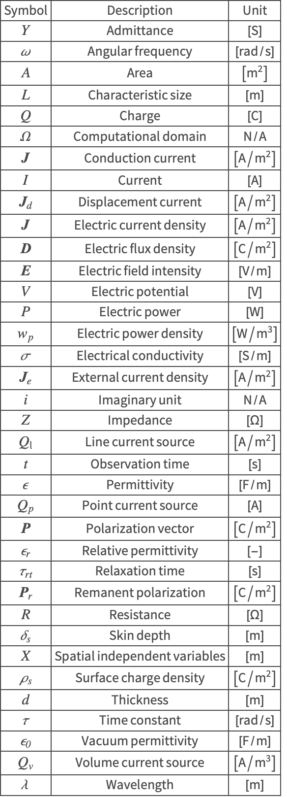
References
1. Agarwal, A. and Lang, J. (2018). Foundations of Analog and Digital Electronic Circuits (2nd ed.). Morgan Kaufmann.
2. Bilbao, S. and Hamilton, B. (2017, October). "Directional Source Modeling in Wave-Based Room Acoustics Simulation." In 2017 IEEE Workshop on Applications of Signal Processing to Audio and Acoustics (WASPAA) (pp. 121–125). IEEE.
3. Cardoso, J. R. (2018). Electromagnetics through the Finite Element Method. Boca Raton: CRC Press.
4. Peskin, C. S. (2002). "The Immersed Boundary Method." Acta Numerica, 11, pp. 479–517.
5. Sadiku, M. N. O. (2011). Elements of Electromagnetics (5th ed.). Oxford University Press.