

PredictorMeasurements
PredictorMeasurements[predictor,testset,prop]
predictor が testset について評価されたときに,特性 prop に関連する測度を与える.
PredictorMeasurements[predictor,testset]
任意の特性に適応可能な測定報告を与える.
PredictorMeasurements[data,…]
予測器の代りに予測 data を使う.
PredictorMeasurements[…,{prop1,prop2,…}]
特性 prop1,prop2等を与える.
詳細とオプション
- 測定は,訓練目的で使われたものではないデータ(検定集合)に対する予測器の性能を決定するために使われる.
- 使用可能な測定方法には,分類測定(確度,尤度等),可視化(混同行列,ROC曲線など),特定の例(最悪の分類例等)がある.
- predictor は,一般に,Predictによって生成されるPredictorFunctionオブジェクトである.
- PredictorMeasurements[data,…]の予測 data は次の形でよい.
-
{y1,y2,…} 予測器(人間,アルゴリズム等)からの予測 {dist1,dist2,…} 予測器によって入手された予測分布 - PredictorMeasurements[…,opts]は,検定集合に適用される場合に,予測器がオプション opts を使うように指定する.使用可能なオプションは,PredictorFunctionで与えられるものと同じである.
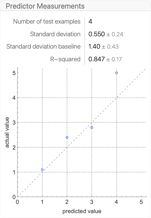
- PredictorMeasurements[predictor,testset]は,以下のような報告パネルを表示するPredictorMeasurementsObject[…]を返す.
- PredictorMeasurementsObject[…][prop]を使ってPredictorMeasurementsObject中の prop を検索することができる.繰り返し特性を検索することが必要な場合は,これの方がPredictorMeasurementsを毎回使うよりも一般により効率がよい.
- PredictorMeasurementsObject[…][prop,opts]は,検定集合に適用される場合に,予測器がオプション opts を使うように指定する.これは,PredictorMeasurementsに与えられたもとのオプションに優先する.
- PredictorMeasurementsには,PredictorFunction[…]のオプションに次を加えたものが使える.
-
Weights Automatic 検定集合例と関連した重み ComputeUncertainty False 尺度をその不確実性とともに与えるかどうか - ComputeUncertaintyTrueの設定のとき,数値測度値はAround[result,err]として返される.err は測定結果 result に関連付けられた(68%信頼区間に相当する)標準誤差を表す.
- 次はWeightsの可能な設定である.
-
Automatic 重み1とすべての検定例を関連付ける {w1,w2,…} 重み wiと i  番目の検定例を関連付ける
 - 検定例の重みを1から2に変更することは,例を重複することに等しい.
- 重みは測度値とその不確定性に影響する.
- 次は,検定集合について予測能力に関連した単一の数値を返す特性である.
-
"StandardDeviation" 剰余の二乗平均平方根 "StandardDeviationBaseline" 検定集合の値の標準偏差 "LogLikelihood" 検定データを与えられた場合の,モデルの対数尤度 "MeanCrossEntropy" 検定例に対する平均クロスエントロピー "MeanDeviation" 剰余の絶対値の平均 "MeanSquare" 剰余の平方の平均 "RSquared" 決定係数 "FractionVarianceUnexplained" 原因不明の分散の割合 "Perplexity" 平均クロスエントロピーの指数 "RejectionRate" Indeterminateとして予測された例の割合 "GeometricMeanProbabilityDensity" 実クラス確率密度の幾何平均 - Indeterminateと分類された検定例は,"StandardDeviation"や"MeanCrossEntropy"のような,検定集合についての予測能力に関連した特性を計測する際には破棄される.
- 次は,グラフィックスを返す特性である.
-
"ComparisonPlot" 予測値と検定値のプロット "ICEPlots" 個別条件付き期待値(ICE)プロット "ProbabilityDensityHistogram" 実際のクラス確率のヒストグラム "Report" 主な測定値をレポートするパネル "ResidualHistogram" 剰余のヒストグラム "ResidualPlot" 剰余のプロット "SHAPPlots" 各クラスのシャープレイ加法機能の説明プロット - 次は,時間に関連した特性である.
-
"EvaluationTime" 検定集合の1つの例を予測するのにかかった時間 "BatchEvaluationTime" バッチの1つの例を予測するための限界時間 - 次は,各検定集合例に対して1つの値を返す特性である.
-
"Residuals" 予測値と検定値の差のリスト "ProbabilityDensities" 実クラスの予想確率密度 "SHAPValues" 各例についてのシャープレイ加算特徴の説明 - "SHAPValues"は,さまざまな特徴を削除し次に合成した結果の予測を比較することで特徴の貢献度を評価する.オプションMissingValueSynthesisを使って欠測値を合成する方法が指定できる.SHAPの説明は訓練出力の平均からの偏差として与えられる."SHAPValues"n を使ってSHAPの説明の数値推定に使われるサンプル数が制御できる.
- 次は,検定集合からの例を返す特性である.
-
"BestPredictedExamples" 実クラス確率密度が最も高い例 "Examples" すべての検定例 "Examples"{i1,i2} 区間 i2で予想された,区間 i1内のすべての例 "LeastCertainExamples" 分布エントロピーが最も高い例 "MostCertainExamples" 分布エントロピーが最も低い例 "WorstPredictedExamples" 実クラス確率密度が最も低い例 - 例は inputivalueiの形で与えられる.valueiは実際の値である.
- "WorstPredictedExamples"や"MostCertainExamples"のような特性は10例まで出力する.PredictorMeasurementsObject[…][propn]を使って出力数を n 例に指定することができる.
- 次は,その他の特性である.
-
"PredictorFunction" 測定されているPredictorFunction[…] "Properties" 使用可能な測度特性のリスト
例題
すべて開く すべて閉じる例 (3)
p = Predict[{1 -> 2, 3 -> 4.5, 5 -> 6, 7 -> 8.5}]testset = {1.5 -> 2, 4 -> 5, 6 -> 5.5};PredictorMeasurements[p, testset, "StandardDeviation"]PredictorMeasurements[p, testset, "ResidualPlot"]PredictorMeasurements[p, testset, "ComparisonPlot"]PredictorMeasurements[p, testset, {"StandardDeviation", "RSquared", "MeanCrossEntropy"}]p = Predict[{1 -> 2, 3 -> 4.5, 5 -> 6, 7 -> 8.5}]pm = PredictorMeasurements[p, {1.5 -> 2, 4 -> 5, 6 -> 5.5}]pm["Properties"]pm["StandardDeviation"]標準偏差を有限な検定集合サイズによる統計的不確かさとともに入手する:
pm["StandardDeviation", ComputeUncertainty -> True]pm[{"StandardDeviation", "RSquared"}, ComputeUncertainty -> True]PredictorMeasurements[{1, 2, 3, 4}, {1.1, 2.4, 2.8, 5}, "StandardDeviation"]PredictorMeasurements[{1, 2, 3, 4}, {1.1, 2.4, 2.8, 5}]PredictorMeasurements[{NormalDistribution[1, 1.2], NormalDistribution[2, 0.8], NormalDistribution[3, 1.9], NormalDistribution[4, 2.1]}, {1.1, 2.4, 2.8, 5}, "LogLikelihood"]スコープ (3)
残差に基づく測定 (1)
PredictorMeasurements[{1, 2, 3, 4}, {1.1, 2.4, 2.8, 5}, "ResidualPlot"]PredictorMeasurements[{1, 2, 3, 4}, {1.1, 2.4, 2.8, 5}, "StandardDeviation"]Sqrt@Mean[PredictorMeasurements[{1, 2, 3, 4}, {1.1, 2.4, 2.8, 5}, "Residuals"] ^ 2]PredictorMeasurements[{1, 2, 3, 4}, {1.1, 2.4, 2.8, 5}, "StandardDeviation", ComputeUncertainty -> True]標準偏差を(常に検定集合の値の平均を予測する)ベースラインと比較する:
PredictorMeasurements[{1, 2, 3, 4}, {1.1, 2.4, 2.8, 5}, "StandardDeviationBaseline", ComputeUncertainty -> True]
PredictorMeasurements[{1, 2, 3, 4}, {1.1, 2.4, 2.8, 5}, "RSquared"]1 - PredictorMeasurements[{1, 2, 3, 4}, {1.1, 2.4, 2.8, 5}, "StandardDeviation"] ^ 2 / PredictorMeasurements[{1, 2, 3, 4}, {1.1, 2.4, 2.8, 5}, "StandardDeviationBaseline"] ^ 2PredictorMeasurements[{1, 2, 3, 4}, {1.1, 2.4, 2.8, 5}, "FractionVarianceUnexplained"]PredictorMeasurements[{1, 2, 3, 4}, {1.1, 2.4, 2.8, 5}, "RSquared"] + PredictorMeasurements[{1, 2, 3, 4}, {1.1, 2.4, 2.8, 5}, "FractionVarianceUnexplained"]比較プロットと例の抽出 (1)
ボストンの住宅データについての訓練集合と検定集合を作成する:
{training, test} = TakeDrop[RandomSample@ResourceData["Sample Data: Boston Homes"], 300];Dataset[training, MaxItems -> 5]p = Predict[training -> "MEDV"]この分類器についての分類器測定オブジェクトを検定集合について作成する:
pm = PredictorMeasurements[p, test]pm["WorstPredictedExamples" -> 2]#1 -> p[#1]&@@@pm["WorstPredictedExamples" -> 2]pm["BestPredictedExamples" -> 2]#1 -> p[#1]&@@@pm["BestPredictedExamples" -> 2]pm["ComparisonPlot"]真の値が30から40の間の例と予測の値が40から50の間の例を抽出する:
pm["Examples" -> {{30, 40}, {40, 50}}]確率的測定 (1)
式Cos[x*y]から人工的なデータ集合を作成し,可視化する:
Plot3D[Cos[x * y], {x, -2, 2}, {y, -2, 2}]points = {##, Cos[#1 * #2] + RandomReal[{-.2, .2}]}&@@@RandomReal[{-2, 2}, {1000, 2}];ListPointPlot3D[points]{trainingset, testset} = TakeDrop[{#1, #2} -> #3&@@@points, 800];p = Predict[trainingset]検定集合(実際の値の対数-確率密度関数の合計)の対数尤度を測定する:
PredictorMeasurements[p, testset, "LogLikelihood"]PredictorMeasurements[p, testset, "MeanCrossEntropy"]-PredictorMeasurements[p, testset, "LogLikelihood"] / Length[testset]オプション (5)
IndeterminateThreshold (1)
points = {#, Cos[#] + RandomReal[#]}& /@ RandomReal[{-3, 3}, {1000}];
dataset = Rule @@@ points;ListPlot[points]trainingset = dataset[[ ;; 800]];
testset = dataset[[801 ;; ]];p = Predict[trainingset]Plot[{
PDF[p[-2, "Distribution"], y],
PDF[p[-1, "Distribution"], y],
PDF[p[0., "Distribution"], y]
}, {y, -3, 2}, PlotRange -> All, PlotLegends -> "Expressions"]PredictorMeasurements[p, testset, "StandardDeviation"]PredictorMeasurements[p, testset, "StandardDeviation", IndeterminateThreshold -> 1]この操作はPredictorMeasurementsObjectについても行うことができる:
pm = PredictorMeasurements[p, testset]pm["StandardDeviation", IndeterminateThreshold -> 1]Get["MachineLearning`"]
DiscretePlot[pm["StandardDeviation", IndeterminateThreshold -> x], {x, 0, 5, .5}, Joined -> True]DiscretePlot[pm["RejectionRate", IndeterminateThreshold -> x], {x, 0, 5, .5}, Joined -> True]TargetDevice (1)
trainingData = RandomReal[1, {2000, 4}] -> RandomReal[1, 2000];
predictor = Predict[trainingData, Method -> "NeuralNetwork"]TargetDeviceのさまざまな設定について,検定集合についての予測器の標準偏差を測定する:
testset = RandomReal[1, {10, 4}] -> RandomReal[1, 10];AbsoluteTiming[PredictorMeasurements[predictor, testset, "StandardDeviation", TargetDevice -> "GPU"]]AbsoluteTiming[PredictorMeasurements[predictor, testset, "StandardDeviation", TargetDevice -> "CPU"]]UtilityFunction (1)
trainingset = {1 -> 1.1, 2 -> 4.4, 3 -> 6.1, 4 -> 7.1, 5 -> 9.2};testset = {0.7 -> 1.3, 2.1 -> 4.7, 3.5 -> 5.8, 3.5 -> 6.6};p = Predict[trainingset]予測された値が実際の値よりも小さかった場合にペナルティを課す効用関数を定義し,可視化する:
utility[a_, p_] := -Piecewise[{{Exp[p - a], a < p}, {Exp[3 * (a - p)], a ≥ p}}]Plot[utility[0, p], {p, -1, 2}]この効用関数を使って,検定集合についての予測器の剰余を計算する:
PredictorMeasurements[p, testset, "Residuals", UtilityFunction -> utility]PredictorMeasurements[p, testset, "Residuals"]この効用関数は,PredictorMeasurementsObjectを使った場合にも指定することができる:
pm = PredictorMeasurements[p, testset]pm["Residuals", UtilityFunction -> utility]"Uncertainty" (1)
"WineQuality"データ集合について予測器を訓練する:
training = ExampleData[{"MachineLearning", "WineQuality"}, "TrainingData"];p = Predict[training]検定集合を使ってPredictorMeasurements[…]オブジェクトを生成する:
test = ExampleData[{"MachineLearning", "WineQuality"}, "TestData"];pm = PredictorMeasurements[p, test]pm["StandardDeviation", ComputeUncertainty -> True]Dataset[AssociationMap[pm[#, ComputeUncertainty -> True]&, {"GeometricMeanProbabilityDensity", "MeanCrossEntropy", "MeanDeviation", "MeanSquare", "TotalSquare"}]]Weights (1)
p = Predict[{1 -> 2, 3 -> 4.5, 5 -> 6, 7 -> 8.5}]各検定例が持つ重みを指定しながら測度オブジェクトを生成する:
pm = PredictorMeasurements[p, {1.5 -> 2, 4 -> 5, 6 -> 5.5, 3 -> 5}, Weights -> {1.5, 3, 2, 1}]pm["StandardDeviation"]pm["StandardDeviation", Weights -> {1, 1, 1, 3}]pm["StandardDeviation", ComputeUncertainty -> True]pm["StandardDeviation", Weights -> {1, 1, 1, 3}, ComputeUncertainty -> True]アプリケーション (2)
月平均気温のデータ集合を,都市,年,月の関数としてのロードする:
dataset = RandomSample[{#2, #3, #4} -> #1& @@@ExampleData[{"Statistics", "USCityTemperature"}]];RandomSample[dataset, 3] // TableFormtrainingset = dataset[[ ;; 200]];testset = dataset[[201 ;; ]];p = Predict[trainingset]予測器と検定集合からPredictorMeasurementsObjectを生成する:
pm = PredictorMeasurements[p, testset]検定集合に対しての分類器の平均クロスエントロピーを計算する:
pm["MeanCrossEntropy"]pm["ComparisonPlot"]pm["Examples" -> {{30, 40}, {40, 60}}]pm["WorstPredictedExamples" -> 20]ある地区の特徴を与えられた場合に,ボストンのその地区における住宅価値の中央値を予測する予測器を訓練する:
p = Predict[ExampleData[{"MachineLearning", "BostonHomes"}, "TrainingData"], PerformanceGoal -> "Quality"]予測器測度を生成し,検定集合についての予測器のパフォーマンスを分析する:
pm = PredictorMeasurements[p, ExampleData[{"MachineLearning", "BostonHomes"}, "TestData"]]pm["ResidualPlot"]pm["ResidualHistogram"]実際の値(剰余の二乗平均平方根)から予測値の標準偏差を計算する:
pm["StandardDeviation"]pm["StandardDeviation", ComputeUncertainty -> True]テキスト
Wolfram Research (2014), PredictorMeasurements, Wolfram言語関数, https://reference.wolfram.com/language/ref/PredictorMeasurements.html (2021年に更新).
CMS
Wolfram Language. 2014. "PredictorMeasurements." Wolfram Language & System Documentation Center. Wolfram Research. Last Modified 2021. https://reference.wolfram.com/language/ref/PredictorMeasurements.html.
APA
Wolfram Language. (2014). PredictorMeasurements. Wolfram Language & System Documentation Center. Retrieved from https://reference.wolfram.com/language/ref/PredictorMeasurements.html