SystemModelSimulateSensitivity

SystemModelSimulateSensitivity[model,{p₁,p₂,…}]

simulates model and sensitivities to parameters p_i following experiment settings.

SystemModelSimulateSensitivity[model,t_max,{p₁,p₂,…}]

simulates from 0 to t_max.

SystemModelSimulateSensitivity[model,{t_min,t_max},{p₁,p₂,…}]

simulates from t_min to t_max.

SystemModelSimulateSensitivity[model,vars,{t_min,t_max},{p₁,p₂,…}]

stores only simulation data for the variables vars.

Details and Options

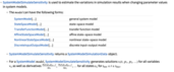
SystemModelSimulateSensitivity is used to estimate the variations in simulation results when changing parameter values in system models.
The model can have the following forms:

	SystemModel[…]	general system model
	StateSpaceModel[…]	state-space model
	TransferFunctionModel[…]	transfer function model
	AffineStateSpaceModel[…]	affine state-space model
	NonlinearStateSpaceModel[…]	nonlinear state-space model
	DiscreteInputOutputModel[…]	discrete input-output model

SystemModelSimulateSensitivity returns a SystemModelSimulationData object.
For a SystemModel model, SystemModelSimulateSensitivity generates solutions for all variables , as well as derivatives , , … for all states , for .
For other types of models, SystemModelSimulateSensitivity generates solutions for all variables , as well as derivatives , , …, for .
Sensitivities can be listed in a SystemModelSimulationData object sd with sd["SensitivityNames"].
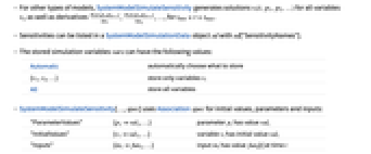
The stored simulation variables vars can have the following values:
Automatic automatically choose what to store

{v₁,v₂,…} store only variables v_i

All store all variables
SystemModelSimulateSensitivity[…,spec] uses Association spec for initial values, parameters and inputs:

"ParameterValues"	{p₁val₁,…}	parameter p_i has value val_i
"InitialValues"	{v₁val₁,…}	variable v_i has initial value val_i
"Inputs"	{in₁fun₁,…}	input in_i has value fun_i[t] at time t

Setting "ParameterValues" or "InitialValues" to {p_i->{c₁,c₂,…},…} runs simulations in parallel, with p_i taking values c_j.
"InitialValues" corresponds to the start property in the Modelica model.
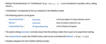
The following options can be given:

InterpolationOrder	Automatic	continuity degree of output between events
Method	Automatic	what simulation method to use
ProgressReporting	$ProgressReporting	control display of progress

The option setting Automatic normally means that the setting is taken from model or its experiment setting.
For a SystemModel model, the CVODES solver used can be controlled with Method->{"opt₁"->val₁}.
Possible suboptions for the CVODES method include:
"InterpolationPoints" Automatic number of interpolation points

"Tolerance" 10⁶ tolerance for adaptive step size

Examples

open allclose all

Basic Examples (3)

Study sensitivity of a parameter over the time interval in model experiment settings:

Extract sensitivity names and plot them:

Show the sensitivity of a signal to relative changes in a parameter:

Plot bounds for y and z when varying a by 10%:

Use the diagram representation of a model as input:

Copy and paste the output above:

Scope (16)

Models (3)

Compute variables and sensitivities when simulating a NonlinearStateSpaceModel:

Extract sensitivity names and plot them:

Plot bounds for a state when varying a by 40%:

Compute sensitivities in a parameter sweep for an AffineStateSpaceModel:

Plot bounds for a state when varying a by 50%:

Compute sensitivities for a DiscreteInputOutputModel:

Plot bounds for the output when varying a by 5%:

Simulation Time (3)

Simulate with settings from the model:

Simulate from time 0 to 5:

Simulate for an explicit time interval:

Sensitivity Results (6)

Study the sensitivity of one parameter:

Simulate with sensitivity to parameter a:

Get the sensitivity names:

Get the sensitivity y has to changes in a:

Study the sensitivities from one parameter:

Plot one of the sensitivities:

Show the sensitivity of a signal to a parameter a:

Get the sensitivity names:

Get the sensitivity y has to changes in a, as well as the nominal trajectory for y:

Plot y with original parameter a, and with parameter a increased by 0.05:

Show the sensitivity of a signal to relative changes in a parameter:

Get the sensitivity names:

Get the sensitivity y and z have to changes in a, as well as nominal trajectories and value:

Plot bounds for y and z when varying a by 10% of the sensitivity:

Show the sensitivity of a signal to absolute changes in a parameter a:

Get the sensitivity y has to changes in a, as well as the trajectory for y:

Compute the change in y when parameter a changes with absolute value 0.1:

Plot the variation of y when parameter a varies by ±0.1:

Variables, Parameters and Inputs (3)

Change the initial values of a simulation:

Compare the changes in a plot:

Change the parameter values of a simulation:

Compare the two in a plot:

Give an input function for a variable and study the sensitivity of the output to a gain parameter:

Plot the sensitivity of the output to the gain parameter:

Result Storage (1)

Store only selected variables:

Only the given variables and parameters are saved:

Generalizations & Extensions (1)

Debug messages are collected in the message group "WSMDebug":

Turn on debug messages for initialization:

Turn off all debug messages for "WSMDebug":

Options (3)

InterpolationOrder (1)

Simulate with interpolation orders 1 and 3, and 3 interpolation points:

Show the sensitivity variable:

Method (1)

Simulate a SystemModel and compute sensitivities with the number of interpolation points set by the model:

Simulate and compute sensitivities with a custom number of interpolation points:

ProgressReporting (1)

Control progress reporting with ProgressReporting:

Applications (5)

Study the sensitivity of a model:

Get the value of the parameter:

Find the peak deviation when varying the parameter:

Show a 5% sensitivity bound and the peak deviation time:

Find out which variable is most sensitive to a frequency parameter:

A 10% sensitivity bound shows that "integrator3.y" is most sensitive to the parameter:

Simulate a rolling wheel:

Select the position of the wheel and its sensitivities to different parameters:

Show the path of the wheel with 4% variation of the wheel radius and mass, respectively:

Calibrate parameters in a model by comparing to measurement data:

Set up caching for simulation:

Use SystemModelSimulateSensitivity to get gradients:

Plot the result of the simulation for specific parameter values:

Fit parameters to the measurement data:

Not using gradients takes longer:

Simulate with the fitted parameters:

Show the test data and the calibrated model together:

Plot a solution with its sensitivity bounds:

Get the nominal value of the parameter:

Show a 5% sensitivity bound:

Simulate with a maximal variation of 5%:

Get the trajectories:

Show that the trajectories are mostly contained in the approximated sensitivity bounds:

Properties & Relations (4)

Compare a sensitivity simulation with the sensitivity of the corresponding differential equation:

Plot bounds for a relative parameter change:

Get the sensitivity y has to changes in a, as well as y and the value for a:

Plot bounds for y when varying a by 10% of the sensitivity:

Use SystemModelPlot instead:

Sensitivities are valid for small changes in the parameter:

Get sensitivities to a parameter:

Simulate with variation of the parameter:

Comparing in a plot, a 10% variation gives trajectories outside computed bounds:

Use SystemModelParametricSimulate for a function that can be evaluated for different values:

Compute solutions for different values of the frequency parameter:

Plot the solutions over time:

Neat Examples (1)

Show sensitivity bounds for the and axes in the Rabinovich–Fabrikant equations:

Show the sensitivity bounds in 3D:

Top

SystemModelSimulateSensitivity

Details and Options

Examples

Basic Examples (3)